Eigenvalues of Tree Graph

This blog version is slightly incomplete compared to the pdf version on github. I put all related code there too.

Introduction

The Laplacian of \(G\) is defined as \(Q = D - M\), where \(D\) is the diagonal matrix of outdegrees of vertices and \(M\) is the adjacency matrix of \(G\).

An \(l\)-walk, or \(l\)-path, in a directed graph \(G=(V,E)\) means a directed \(l\)-walk, that is a sequence \((u_0,e_1,u_1,\cdots ,e_{l}, u_l)\) of vertices and edges of \(G\) such that for each \(1\leqslant i\leqslant l\), edge \(e_i\) has initial vertex \(u_{i-1}\) and terminal vertex \(u_i\). The walk is closed if \(u_0=u_l\).

If \(S\) is a nonempty subset of \(V\), we denote by \(G_{S}\) the induced subgraph of \(G\) on the vertex set \(S\), that is the directed graph obtained from \(G\) by only keeping vertices in \(S\) and edges with both endpoints in \(S\).

tree graph

In this section we recall some basic concepts and introduce a few previous results.

Spanning trees and forests

Let \(G = (E,V)\) be a finite directed graph. For each edge we denote \(s(e)\) its source and \(t(e)\) its target. A (rooted) spanning tree of \(G\) is a subgraph of \(G\) containing all vertices with no cycle. There is one vertex \(r\), called the root, having outdegree \(0\) and the other vertices have outdegree \(1\). By the nature of tree, the spanning tree of \(G\) has \(|V|-1\) edges.

Generally, if $W V $ is a nonempty subset, a forest of \(G\) rooted in \(W\) is defined as the following subgraph: it contains all vertices, with no cycle, and the vertices in \(W\) have outdegree \(0\) while the other vertices have outdegree \(1\).

Tree graph \(\mathcal{T}G\)

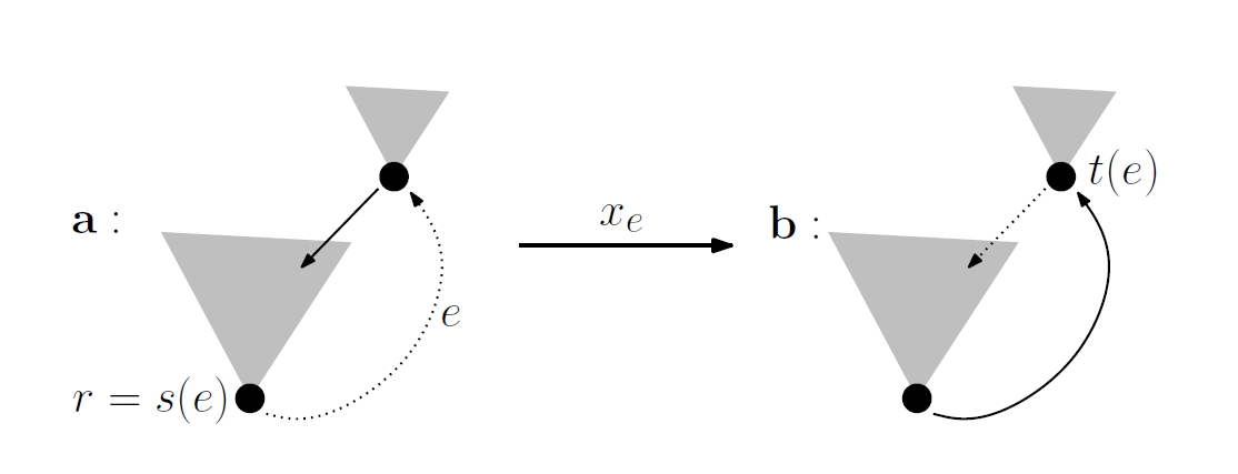
The tree graph of \(G\), denoted \(\mathcal{T}G\), is the directed graph whose vertices are the spanning trees of \(G\) and whose edges are obtained by the following construction:

Let \(\mathbf{a}\) be a spanning tree of \(G\) with root \(r\). For an edge \(e\in E\) with \(s(e)=r\), let \(\mathbf{b}\) be the subgraph of \(G\) obtained by adding edge \(e\) to \(\mathbf{a}\) then deleting the edge coming out of \(t(e)\) in \(\mathbf{a}\).

It's easy to check that \(\mathbf{b}\) is a spanning tree of \(G\), with root \(t(e)\).

In the following we will denote \(\mathcal{T}V\) the set of vertices of \(\mathcal{T}G\), i.e., the set of spanning trees of \(G\).

There is a natural map \(p\) from \(\mathcal{T}G\) to \(G\). \(p\) maps each vertex of \(\mathcal{T}G\) to its root, and maps each edge of \(\mathcal{T}G\) to the edge \(e\) of \(G\) for its construction.

Now we give here some elementary properties of the tree graph. See previous papers for proofs.

• \(\mathcal{T}G\) is simple and has no loop.
• The graph \(\mathcal{T}G\) is strongly connected if \(G\) is.
• The graph \(\mathcal{T}G\) is a covering graph of \(G\).
• The set of edges of \(\mathcal{T}G\) can be partitioned into edge-disjoint simple cycles, which project onto simple cycles of \(G\). If \(C\) is a simple cycle of \(G\), with vertex set \(W\), then the number of simple cycles of \(\mathcal{T}G\) lying above \(C\) is equal to the number of forests rooted in \(W\).
• The graph \(\mathcal{T}G\) is Eulerian: The number of outgoing or incoming edges of a vertex \(\mathbf{a}\) are both equal to the number of outgoing edges of the root of \(\mathbf{a}\) in \(G\).

If $W V $, The matrix-tree theorem gives the generating function of spanning forests of \(G\) rooted in \(W\) . Moreover, it's easy to know the total number of those spanning forests: Denote \(Q^{W}\) as the matrix obtained from the Laplacian matrix \(Q\) of \(G\) by deleting rows and columns indexed by elements of \(W\), then the number of spanning forests of \(G\) rooted in \(W\) is given by \(\det (Q^{W})\).

In particular, let \(W = \{r\}\), then the number of spanning trees of \(G\) rooted in \(r\) is given by \(\det (Q^{r})\). For convenience in the following we use the notation \(Q_{W} = Q^{V \backslash W}\) to denote the matrix extracted from the Laplacian matrix \(Q\) of \(G\) by keeping only rows and columns indexed by elements of \(W\).

It is important to notice that the matrix-tree theorem is valid for both directed and undirected graphs.

By the matrix-tree theorem, we can easily derive all spanning trees of \(G\), then construct the tree graph \(\mathcal{T}G\).

Eigenvalues of Tree Graph

Though astonishing, eigenvalues of the adjacency matrix of the tree graph \(\mathcal{T}G\) can be computed explicitly. This can be expected from the following fact: the \((i,j)\) entry of the matrix \(M\), where \(M\) is the adjacency matrix of \(G\), equals the number of \(l\)-walks in \(G\) which start at \(v_i\) and end at \(v_j\). Thus, the number of closed \(l\)-walks in \(\mathcal{T}G\), which we will denote by \(w(\mathcal{T}G, l)\), equals the trace of \(M^{l}\) and hence the sum of the \(l\)th powers of the eigenvalues of \(M\).

C. Athanasiadis proved the following theorem about eigenvalues of \(\mathcal{M}\), i.e., the adjacency matrix of \(\mathcal{T}G\).

In Biane and Chapuy's paper, they wrote the theorem wrongly (Proposition 3.1)

Theorem The nonzero eigenvalues of \(\mathcal{M}\) are eigenvalues of \(M_{X};X \subseteq V\) where \(M\) is the adjacency matrix of \(G\). For an eigenvalue \(\gamma\), let \(m_{X}(\gamma)\) denotes its multiplicity in \(M_{X}\), then its multiplicity in \(\mathcal{M}\) is \[ \sum_{X \subseteq V }^{} m_{X}(\gamma) \det(Q_{V\backslash X}-I) \]

Here we make the convention that \(\det(Q_{\emptyset}-I) = 1\).

The original proof from Athanasiadis is a little confusing, so we make it more clear here. First we need to calculate \(w(\mathcal{T}G,l)\).

Theorem For a directed graph \(G\) on the vertex set \(V\) we have \[ w(\mathcal{T}G, l) = \sum_{S \subseteq V} w(G_{S}, l) \det(Q_{V\backslash S}-I). \]

proof A closed \(l\)-walk in \(\mathcal{T}G\) is determined by a spanning tree \(T_0\) on \(G\) with root \(r\), and a closed \(l\)-walk \(W=(u_0,e_1,u_1,\cdots ,e_l,u_l)\) in \(G\) with \(u_0=u_l=r\). Let \(a=(u_0,u_1,\cdots ,u_l)\). The sequence \(a\) determines the roots of the trees \(T_0, T_1,\cdots ,T_{l}=T_0\) to be visited during the walk in \(\mathcal{T}G\).

Fix a closed \(l\)-walk \(W\) in \(G\) together with the sequence \(a\). Following Athanasiadis's argument (Theorem 2.2) the number of trees \(T_0\) which will yield a closed \(l\)-walk in \(\mathcal{T}G\) is the number \(\tau(G,U)\) of spanning forests on \(G\) with root set \(U=\{u_0,u_1,\cdots ,u_l\}\). Finally, the number of closed \(l\)-walks in \(\mathcal{T}G\) is \[ w(\mathcal{T}G,l) = \sum_{U \subseteq V }^{} g(G_{U},l)\tau(G,U), \]

where \(g(G,l)\) stands for the number of closed \(l\)-walks in a graph \(G\) visiting all of its vertices.

We may explain (1) more explicitly. Notice that a closed \(l\)-walk in \(G\) can have repeated vertices, so if \(G_{U}\) has a closed \(l\)-walk visiting all of its vertices, then \(\lvert U \rvert\) can be divided by \(l\). Also, \(G_{U}\) can have more than one closed \(l\)-walk. The inclusion-exclusion principle gives \[ g(G_{U},l) = \sum_{S\subseteq U }^{} (-1)^{\lvert U-S \rvert }w(G_{S},l). \]

Hence, after using (2) to compute \(g(G_{U},l)\) and changing the order of summation, (1) becomes \[ w(\mathcal{T}G,l) = \sum_{S\subseteq V }^{} w(G_{S},l) \sum_{S \subseteq U \subseteq V }^{} (-1)^{\lvert U-S \rvert }\tau(G,U). \]

Recall that by the matrix-tree theorem, \(\tau(G,U) = \det(Q_{V\backslash U})\), thus \[ w(\mathcal{T}G,l) = \sum_{S \subseteq V} w(G_{S},l)\sum_{S \subseteq U \subseteq V }^{} (-1)^{\lvert U-S \rvert }\det (Q_{V\backslash U}) = \sum_{S \subseteq V} w(G_{S},l)\det(Q_{V\backslash S}-I). \]

Now that we have the number of closed \(l\)-walks in \(\mathcal{T}G\), we can compute the trace of \(\mathcal{M}^{l}\) and \(M^{l}\). We need the following lemma to complete the proof.

lemma Suppose that for some nonzero complex numbers \(a_i\), \(b_j\), where \(1\leqslant i\leqslant r\) and \(1\leqslant j\leqslant s\) we have \[ \sum_{i=1}^{r} a_i^{l} = \sum_{j=1}^{s} b_j^{l} \]

for all positive integers \(l\). Then \(r=s\) and the \(a_i\) are a permutation of the \(b_j\).

The proof can be found in Athanasiadis's paper.

From theorem 3.2 and Lemma 3.3 we immediately get theorem 3.1.

Example of Complete Graph

The complete directed graph \(K_{n}\) is the graph on the vertex set \(V=[n] = \{1,2,\cdots ,n\}\) with exactly one directed edge from \(i\) to \(j\) for each \(i\neq j\).

Eigenvalues of \(\mathcal{T}K_{n}\)

proposition With \(G=K_{n}\), \(n\geqslant 2\), \(\mathcal{M}\) has eigenvalues \(-1, 1,\cdots ,n-1\). The multiplicity of \(i\) is \[ m_{\mathcal{M}}(i) = \begin{cases} i{n \choose i+1}(n-1)^{n-i-2}, \quad 1\leqslant i\leqslant n-1 \\ n^{n-1}-(n-1)^{n-1}, \quad i=-1. \end{cases} \]

proof First we calculate the eigenvalues of \(K_{n}\). Note that \((1,\cdots ,1)^{\mathsf{T}}\) is an eigenvector of \(M\) with eigenvalue \(n-1\). Besides, \(J_n\), the \(n\times n\) matrix with all entries equal to \(1\), has a kernel of dimension \(n-1\). Thus the eigenvalues of \(K_{n}\) are \(n-1\) with multiplicity \(1\) and \(-1\) with multiplicity \(n-1\). Hence, by theorem 3.1, the eigenvalues of \(\mathcal{M}\) are \(-1, 1,\cdots ,n-1\). Moreover the eigenvalue \(m-1\), \(2\leqslant m\leqslant n\) has multiplicity \[ {n \choose m}\det (Q_{V\backslash [m]}-I) = {n \choose m}(m-1)(n-1)^{n-m-1}. \]

which is easy to obtain by consider eigenvalues of \(Q_{V\backslash [m]}-I\).

\(-1\) has multiplicity \[ \begin{aligned} &\sum_{m=2}^{n} {n \choose m}(m-1)\det (Q_{V\backslash [m]}-I) \\ &= \sum_{m=1}^{n} (m-1)^{2} {n\choose m} (n-1)^{n-m-1} = n^{n-1}-(n-1)^{n-1}. \end{aligned} \]

The multiplicities we have so far add up to \(n^{n-1}\), so \(0\) is not an eigenvalue of \(\mathcal{M}\) and the proposition follows.

Properties of \(\mathcal{T}K_{n}\)

Properties of \(K_{n}\) have always been interesting. We have a lot more to say about \(\mathcal{T}K_{n}\). First, since \(\mathcal{T}K_{n}\) is a covering graph of \(K_{n}\), we have the following proposition.

proposition \(\mathcal{T}K_{n}\) is a regular graph where each vertex has outdegree and indegree \(n-1\).

However, we remind readers that while every vertex in \(\mathcal{T}K_{n}\) has outdegree \(n-1\) is obvious from the construction of edges in \(\mathcal{T}K_{n}\), the constant indegree of each vertex is not trivial at all. Given a spanning tree \(T_0\) of \(K_{n}\), writing down all \(T_1,\cdots ,T_{n-1}\) that \(T_i \rightarrow T_0\) in \(\mathcal{T}K_{n}\) is not that easy. The difficulty lies in irreversibility of the construction of edges in \(\mathcal{T}K_{n}\). Actually, we can get the following proposition.

proposition Let \(T_1\) is a spanning tree of \(K_{n}\) with root \(r_1\), \(T_2\) is a spanning tree of \(K_{n}\) with root \(r_2\). There is an edge \(T_1\rightarrow T_2\) in \(\mathcal{T}K_n\). Then there is an edge \(T_2 \rightarrow T_1\) in \(\mathcal{T}K_{n}\) if and only if \(r_2 \rightarrow r_1\) in \(T_1\). Also, by definition, we have \(r_1 \rightarrow r_2\) in \(T_2\). In the remaining we will say that there is a bi-edge between \(T_1\) and \(T_2\).

proof Suppose \(r_2\rightarrow r_1\) in \(T_1\). Then in \(T_2\), we have \(r_1\rightarrow r_2\), and \(r_1\) has no other outgoing edges. Thus, if we add \(r_2 \rightarrow r_1\) in \(T_2\) and delete \(r_1 \rightarrow r_2\) in \(T_2\), we get exactly \(T_1\). Hence, \(T_2 \rightarrow T_1\) in \(\mathcal{T}K_{n}\). Conversely, suppose \(T_2 \rightarrow T_1\) in \(\mathcal{T}K_{n}\). By definition, \(r_2\rightarrow r_1\) in \(T_1\).

From the above proposition, we know that given \(T_0\), the number of \(T\) such that \(T_0\) and \(T\) has a bi-edge equals the indegree of \(r_0\) in \(T_0\), where \(r_0\) is the root of \(T_0\).

For any \(m\), we now consider number of rooted trees with \(m\) bi-edges. There is a helpful simple decomposition of rooted trees: Let \(T\) be a rooted tree. If we remove all edges incident with the root, we get the root together with a set of trees. Number of trees equals indegree of the root.

proposition With \(G=K_{n}\), number of trees with \(m\) bi-edges is \[ nm {n-1 \choose m}(n-1)^{n-2-m} \]

proof First, there are \(n\) choices of root, denoted as \(r_0\). Second, by the above discussion, there are \({n-1\choose m}\) choices of roots after the decomposition, denoted as \(r_1,\cdots ,r_m\). Finally, excluding \(r_0\), number of forests rooted in \(r_1,\cdots ,r_m\) equals to \(\det (n-1)I_{n-1-m}-J_{n-1-m}\), which is \(m(n-1)^{n-2-m}\). By multiplicity principle, we get the proposition.

proposition With \(G=K_n\), if \(T_0\rightarrow T_1\), \(T_1\rightarrow T_2\) in \(\mathcal{T}G\), then \(T_0\nrightarrow T_2\).

proof Denote roots of \(T_0,T_1,T_2\) as \(r_0,r_1,r_2\) and they are distinct. If \(T_0\rightarrow T_1\) and \(T_1\rightarrow T_2\), then \(r_0\rightarrow r_1\rightarrow r_2\). Thus, if we add an edge from \(r_0\) to \(r_2\), the spanning tree we get is different from \(T_2\).

Three Conjectures

Properties of \(\mathcal{T}K_{n}\) are much more than we have discussed. In particular, while eigenvalues of \(\mathcal{T}K_{n}\) have been computed, the Jordan canonical form of \(\mathcal{T}K_{n}\) has not been obtained. By calculating \(n=3,4,5,6\) cases, we make three conjectures here.

conjecture 1 For eigenvalues \(\lambda=1,2,\cdots ,n-1\) of \(\mathcal{T}K_{n}\), the Jordan blocks are all of size \(1\).

conjecture 2 For eigenvalue \(\lambda=-1\), the Jordan blocks are of size \(1,2,\cdots ,n-1\). Moreover, there are exactly \(n-1\) Jordan blocks of size \(n-1\).

conjecture 3 For eigenvalue \(\lambda=-1\), \(\operatorname{rank}((\mathcal{M}+I)^{n-1})=\operatorname{rank}((\mathcal{M}+I)^{n})=\operatorname{rank}((\mathcal{M}+I)^{n+1})=\cdots =(n-1)^{n-1}\).

We hope to prove or falsify these three conjectures later.

Classification of Vertices of \(\mathcal{T}K_{n}\)

In Biane and Chapuy's paper, they obtain the number of spanning trees of \(\mathcal{T}K_{n}\), namely the number of vertices of graph \(\mathcal{T}^{2}K_{n}\): \[ n^{n-2}\prod_{k=1}^{n-1} ((n-k)n^{k-1})^{(k-1)(n-1)^{n-k-1}{n\choose k}} \]

If we want to calculate eigenvalues of \(\mathcal{T}^{2}K_n\), we need first classify vertices of \(\mathcal{T}K_{n}\). By relabeling this reduces to the problem of classifying unlabeled rooted trees with \(n\) vertices. Namely, we only consider number of equivalence classes under graph isomorphism.

There is no simple formula for counting unlabeled trees. Denote \(r(x)\) be the generating function for number of unlabeled rooted trees, i.e., \(r(x)=\sum_{n=1}^{\infty} r_nx^{n}\) where \(r_n\) is the number of unlabeled rooted trees with \(n\) vertices. Then we have the following theorem.

Theorem The generating function \(r(x)\) for unlabeled rooted trees satisfies \[ r(x) = x h[r(x)] = x \exp \left( \sum_{k=1}^{\infty} \frac{r(x^{k})}{k} \right) . \]

Please refer to Gessel's paper for definition for \(h(A(x))\) and proof of this theorem. We find that \[ \begin{aligned} r(x) = x + x^{2} &+ 2x^{3} + 4x^{4} + 9x^{5} + 20 x^{6} + 48x^{7} + 115x^{8} + 286x^{9} \\ &+ 719x^{10} + 1842 x^{11} + 4766x^{12} + 12486x^{13} + 32973x^{14} \\ &+ 87811x^{15} + 235381 x^{16} + 634847x^{17} + 1721159x^{18} \\ &+ 4688676 x^{19} + 1282622x^{20} + 35221832x^{21} + \cdots \end{aligned} \]

These numbers of sequence A000081 in the Online Encyclopedia of Integer Sequences (OEIS).