Network Effects in Neurostimulation (1)

In our project about network effects of neurostimulation, we care about indirect effects of stimulation on the brain. That's reasonable since - there is significant difference between SC and EC. - Clinically, N2 component of cortico-cortical evoked potentials (CCEPs) is observed^[6]

... In addition, we did not primarily consider indirect cortico-subcortico-cortical pathways that would rather be implicated in the later N2 component ... ^[6]

We hope to build a large scale model of cortex, which shows similar 2-hop network effectis with the real data when applying a virtual stimulus. Furthermore, the model is expected to be used to develop a close-loop network control method.

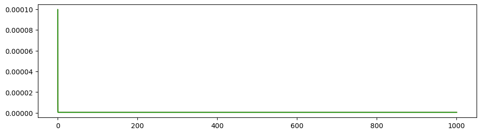
Deco's first model shows poor propagation ratio

The model proposed by Deco^[3] used a dynamical mean field approach to reduce the complexity^[5]. The model is described by the following equations:

\[ \frac{\mathrm{d}S_{i}(t)}{\mathrm{d}t} = -\frac{S_{i}}{\tau_{S}}+ (1-S_i)\gamma H(x_i) +\sigma \nu_i(t) \tag{1} \]

\[ H(x_i) = \frac{ax_{i}-b}{1-\exp (-d(ax_{i}-b))} \tag{2} \]

\[ x_i = wJ_{N}S_i + GJ_{N}\sum_{j}^{} C_{ij}S_{j} + I_0. \tag{3} \]

Here \(H(x_i)\) and \(S_{i}\) denote the population firing rate and the average synaptic gating variable at the loccal cortical area \(i\), hence \(S_{i} \in [0,1]\).

Parameters in (1) - (3) are strongly correlated with dynamics and bifurcation diagram of the model. Heterogeneity across cortices has been considered by Kong^[11], who developed a spatially heterogeneous Deco model. Their aim is to minimize the difference between empirical and simulated FC as well as sharp transitions in FC patterns, which characterized by FCD.

Hard sigmoidal function issue

When doing a simulation of (1) - (3), various numerical methods can be used. We set \(\Delta t = 1 / 2000 s\), which is small enough to avoid stability issue. Hence, we don't worry about using Euler–Maruyama method:

\[ S_i(t+\Delta t) \thickapprox S_i(t) + \left( -\frac{S_i(t)}{\tau_{S}}+(1-S_i(t))\gamma H(x_i) \right) \Delta t + \sigma \xi \sqrt{\Delta t}, \tag{4} \]

where \(\xi \sim \mathcal{N}(0,1)\).

The RHS of (4) can goes negative or larger than 1 regardless of any numerical method (Euler–Maruyama, Runge-Kutta, Exponential-Euler, etc). That is unreasonable, so we applied a hard sigmoidal function: \[ S_i(t+\Delta t) = \min (\max (\text{RHS of (4)}, 0), 1).\tag{5} \]

However, whether to apply the hard sigmoidal function has a significant impact on dynamics.

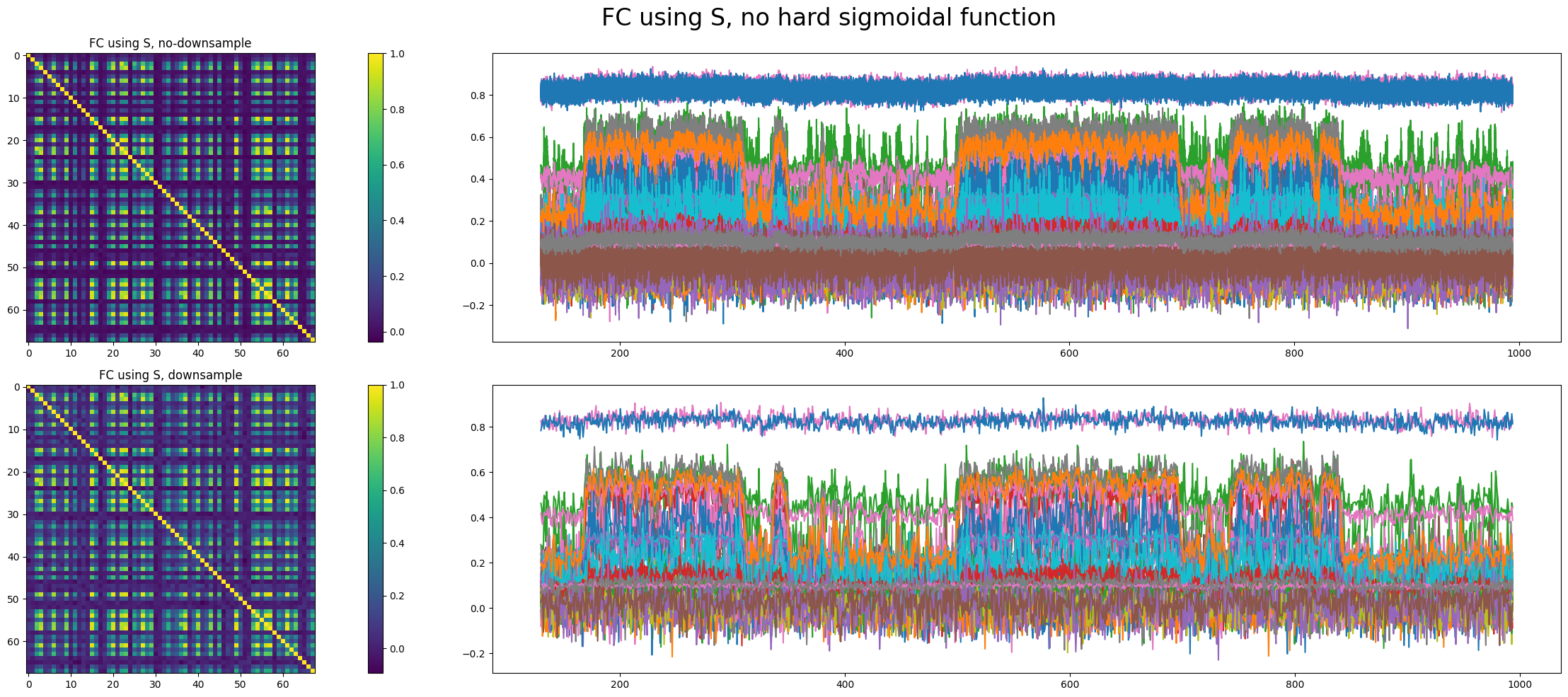
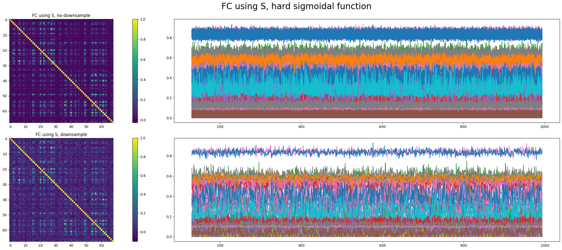
We can see that the network is in a bistable state, one with low activity and the other with relatively high activity. The network makes transitions between these two states.

Multistability is widespread in such nonlinear dynamical systems, one of which impressed me most is bistable states in low-rank RNN^[1][2][8]. If stochasticity is deleted, \(I_0=0, \gamma = 0.641, a = 270, b=108, d=0.154\) as in Deco's paper, RHS of (3) has the value \(6.46 \times 10^{-6}\) when all \(S_i=0\), which is negligible. Given that \(S_i(t)/\tau_{S}\) is linear, \((1-S_i(t))\gamma H(x_i)\) is sub-linear near \(S_i=0\), there indeed exists a low activity stable state.

The real problem is that the high activity state does not correspond to reality since \(S_i\) or \(H(x_i)\) is too large for a resting-state neural network.

Whether to apply the hard sigmoidal function is not decisive in the emergence of transition between two stable states. We found another parameter set that shows such transitions with applying the hard sigmoidal function.

It is mathematically interesting to investigate why adding a hard sigmoidal function reduces the likelihood that the network will switch between two stable states.

Low propagation ratio in Deco's model

We choose to apply the hard sigmoidal function and trained parameters (\(w, \sigma, I_{0}, G\)) based on Kong's code^[11] to suit empirical FC and FCD. The result shows poor correspondence between simulated stimulus time series and real ones, and we think the reason is that the model has a low propagation ratio.

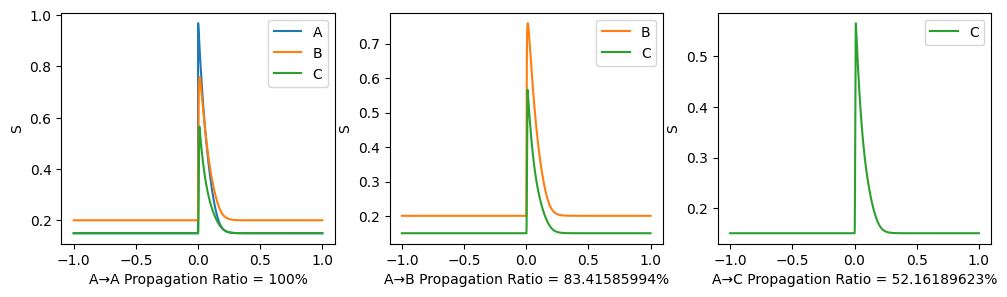
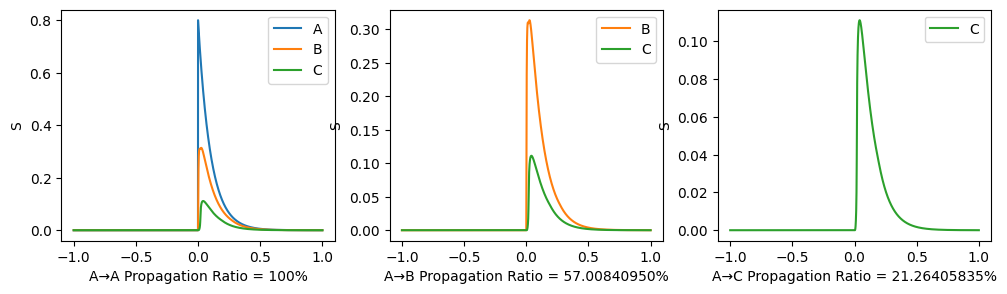
toy model test

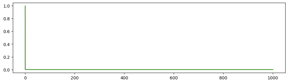
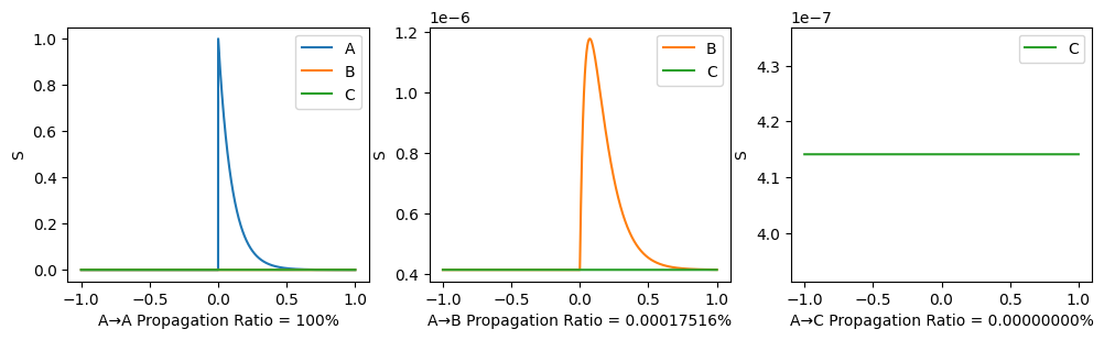
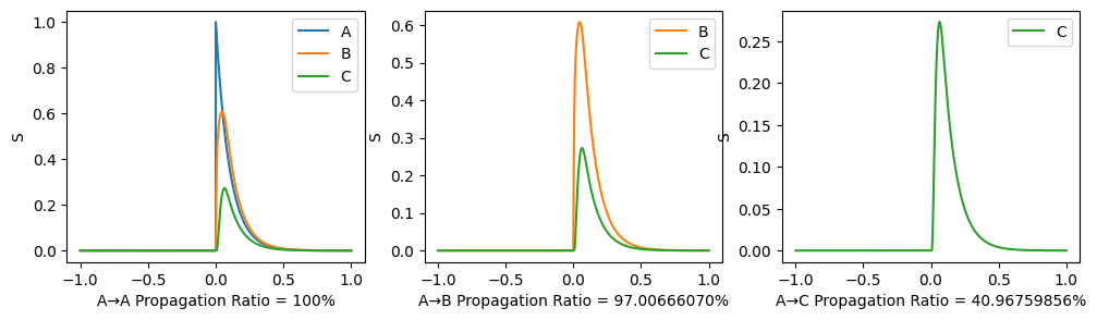
To illustrate the propagation ratio, we use a toy model with only three nodes: A-B-C. The connection for A-B and B-C are the same, while there is no connection between A and C. The structural connectivity matrix is normalized to have spectral radius 0.999. Moreover, noises are deleted, \(I_0\) is set to \(0\) to indicate the propagation more clearly.

After the 3-node model becomes stable (denoted as time 0), a stimulus is applied to node A and we observe its propagation along the path. A→C propagation ratio is defined as \[ \text{A→C propagation ratio} = \frac{\mathbb{E}(S_C(t),t>0)-\mathbb{E}(S_{C}(t), t<0)}{\mathbb{E}(S_{A}(t), t>0)-\mathbb{E}(S_{A}(t),t<0)}. \]

\(G=0.3, w=0.9\) as similar with our trained results:

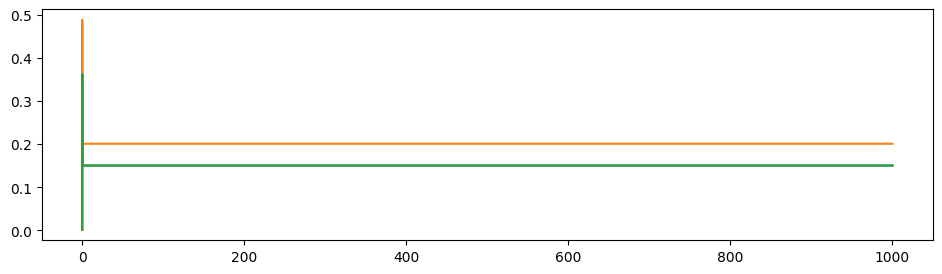
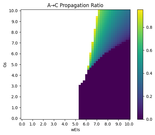
\(G=5.0, w=-2.0\) which is not realistic:

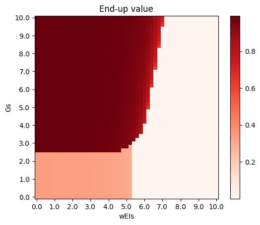
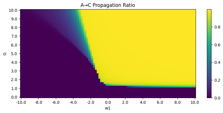
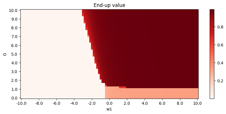
A phase diagram is available:

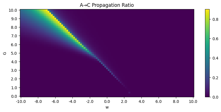
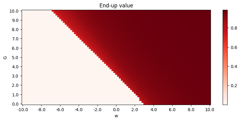
Here, End-up value is the mean of \(S_A, S_B, S_C\) in the end, so a clear phase transition can be seen. The propagation ratio is high only when \(G\) is large and \(w<0\).

Deco's second model shows better propagation ratio

Deco proposed another model^[4] similar to the first one, but with excitatory population and inhibitory population. Heterogeneous version of the model is implemented by Demirtaş et al.^[9] The model is described by the following equations:

\[ \frac{\mathrm{d}S_i^{E}(t)}{\mathrm{d}t} = -\frac{S_i^{E}(t)}{\tau_{E}}+(1-S_i^{E}(t))\gamma H^{E}(x_i^{E}(t)) +\sigma \nu_i(t) \tag{6} \]

\[ \frac{\mathrm{d}S_i^{I}(t)}{\mathrm{d}t} = -\frac{S_i^{I}(t)}{\tau_{I}}+H^{I}(x_i^{I}(t)) +\sigma \nu_i(t) \tag{7} \]

\[ x_i^{E}(t) = w^{E}I_0 + w^{EE}S_i^{E}(t)+gJ_{N} \sum_{j}^{} C_{ij}S_j^{E}(t)-w^{IE}S_i^{I}(t) \tag{8} \]

\[ x_i^{I}(t) = w^{I}I_0 + w^{EI}S_i^{E}(t) - S_i^{I}(t) \tag{9} \]

and \(H^{E}(x_i^{E}), H^{I}(x_i^{I})\) is the same as (2) with different \(a,b,d\). Here, we can regard \(w^{II}=1\).

Deco's model with E-I populations shows boost in propagation ratio in the toy model.

Phase diagrams are as follows (\(G\) versus \(w^{EI}\) as an example, other key parameters: \(w^{EE} = 5, w^{IE} = 1\)), where propagation ratio of high activity endings is deleted:

Though this model exhibits better propagation ratio, the problem is difficulty in model fitting. We are also trying other models.

A possible approach to simplify Deco's model with E-I populations

Demirtaş et al. use parameters as follows:

	Excitatory Populations	Inhibitory Populations
\(I_{0}\)	0.382 nA	-
\(J\)	0.15 nA	-
\(\gamma\)	0.641	-
\(w^{E}\)	1.0	-
\(\tau_{E}\)	0.1 s	-
\(a_{E}\)	310 nC\(^{-1}\)	-
\(b_{E}\)	125 Hz	-
\(d_{E}\)	0.16 s	-
\(w^{I}\)	-	0.7
\(\tau_{I}\)	-	0.01 s
\(a_{I}\)	-	615 nC\(^{-1}\)
\(b_{I}\)	-	177 Hz
\(d_{I}\)	-	0.087 s

Not so strictly, \(\tau_{I} \ll \tau_{E}\), so we can use adiabatic approximation for \(S_i^{I}(t)\), i.e., \(S_i^{I}(t) = \tau_{I}H(x_i^{I}(t))\). With all assumptions aforementioned, (6)-(8) become:

\[ \frac{\mathrm{d}S_i^{E}(t)}{\mathrm{d}t} = -\frac{S_i^{E}(t)}{\tau_{E}}+(1-S_i^{E}(t))\gamma H^{E}(x_i^{E}(t)) \tag{10} \]

\[ x_i^{I}(t) = w^{EI}S_i^{E}(t) - \tau_{I}H^{I}(x_i^{I}(t)) \tag{11} \]

\[ \begin{aligned} x_i^{E}(t) &= w^{EE}S_i^{E}(t)+gJ_{N} \sum_{j}^{} C_{ij}S_j^{E}(t)-w^{IE}\tau_{I}H^{I}(x_i^{I}(t)) \\ &= (w^{EE} - w^{IE}w^{EI})S_i^{E}(t) + gJ_{N}\sum_{j}^{} C_{ij}S_{j}^{E}(t) + w^{IE}x_{i}^{I}(t) \end{aligned} \tag{12} \]

Consider the function: \[ g(x) = x + \tau_{I}\frac{a_{I}x - b_{I}}{1-\exp (-d_{I}(a_{I}x-b_{I}))} = x + 0.01 \frac{615x-177}{1-\exp (-0.087(615x-177))} \tag{13} \]

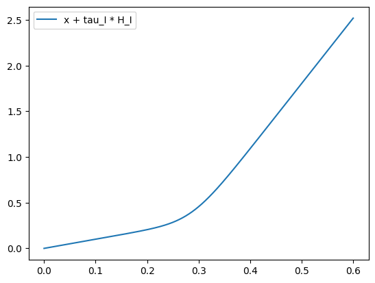
Apart from \(x \in (0.2, 0.32)\), \(g(x)\) can be well approximated by \[ \tilde{g}(x) = \begin{cases} x, \quad x < 177 / 615 \\ x + 0.01 (615x-177), \quad x\geqslant 177 / 615 \end{cases} \]

Hence, (11) has an approximate solution:

\[ \begin{cases} x_i^{I}(t) = w^{EI}S_i^{E}(t), \quad w^{EI}S_{i}^{E}(t)<177/615 \thickapprox 0.288 \\ x_i^{I}(t) = 0.140(w^{EI}S_{i}^{E}(t) + 1.77), \quad w^{EI}S_{i}^{E}(t)\geqslant 0.288 \end{cases} \]

which corresponds to a non-continuous vector field in (12). So a modified Deco model without E-I populations is derived. We only need to check \(S_i^{E}(t)\) every time steps and update \(x_i^{E}(t)\) accordingly.

Adding noise and \(I_0\) back, the model can be described by the following equations: \[ \frac{\mathrm{d}S_i(t)}{\mathrm{d}t} = - \frac{S_i(t)}{\tau_{S}} + (1-S_i(t))\gamma H(x_i(t)) + \sigma \nu_i(t) \tag{14} \]

\[ H(x_i(t)) = \frac{a_{E}x - b_{E}}{1-\exp (-d_{E}(a_{E}x - b_{E}))} \tag{15} \]

\[ x_i(t) = w_0 I_0 + w_1 S_i(t) + gJ_{N}\sum_{j}^{} C_{ij}S_{j}(t) + w_2 y_i(t) \tag{16} \]

\[ y_i(t) = \min(w_3S_i(t) + w_4I_0, (w_3S_{i}(t) + w_4I_0 + 1.77) / 7.15) \tag{17} \]

The modified Deco Model shows good propagation ratio (\(w_0 = 1, w_1 = -3, w_2 = 1, w_3 = 7, w_4 = 0.7, G = 6\)):

Phase diagrams are as follows (\(G\) versus \(w_1\) as an example, other key parameters: \(w_0 = 1, w_2 = 1, w_3 = 7, w_4 = 0.7\)):

To make unit consistent, \(w_1\) can be considered as \(w^{EE}w^{II}-w^{EI}w^{IE}\). Further steps include specification of parameters. \(w_0 = w^{E}\) and \(w_1 = w^{I}\) represent strength of background input, so they are negligible while \(I_0 = 0\). \(w_1 = w^{EE}w^{II} - w^{EI}w^{IE}, w_2=w^{IE}, w_3=w^{EI}, G\) are trainable parameters. Among them \(w_1\) and \(G\) is the key.

More experiments need to be done to verify the effectiveness of this approach.

A resonable explanation for negative w

In (3), negative \(w\) seems not realistic. However, in (12), \(w^{EE}w^{II} - w^{IE}w^{EI}\) is reasonable to be negative, so we can regard negative \(w\) in (3) as a result of E-I balance. That also corresponds with phase diagrams above: when \(w\) is negative and \(G\) is large to compensate for \(w\), the network ends up in a reasonable low activity state and shows high propagation ratio.

Other models

We also apply other models to our project, including vanilla RNN, Joglekar's model^[7], Chaudhuri's model^[10]. Further experiments are expected.

Reference

1. Adrian Valente, Jonanthan W. Pillow. (2022) Extracting computational mechanisms from neural data using low-rank RNNs. NeurIPS. ↩︎
2. Francesca Mastrogiuseppe, Srdjan Ostojic. (2018) Linking Connectivity, Dynamics, and Computations in Low-Rank Recurrent Neural Networks. Neuron. ↩︎
3. Gustavo Deco, Adrián Ponce-Alvarez et al. (2013) Resting-State Functional Connectivity Emerges from structurally and Dynamically Shaped Slow Linear Flunctuations. The Journal of Neuroscience. ↩︎
4. Gustavo Deco, Adrián Ponce-Alvarez et al. (2014) How Local Excitation-Inhibition Ratio Impacts the Whole Brain Dynamics. The Journal of Neuroscience. ↩︎
5. Kong-Fatt Wong, Xiao-Jing Wang. (2006) A Recurrent Network Mechanism of Time Integration in Perceptual Decisions. The Journal of Neuroscience. ↩︎
6. Lemaréchal, Jean-Didier et al. (2022) A brain atlas of axonal and synaptic delays based on modelling of cortico-cortical evoked potentials. Brain. ↩︎
7. Madhura R. Joglekar, Jorge F. Mejias et al. (2018) Inter-areal Balanced Amplification Enhances Signal Propagation in a Large-Scale Circuit Model of the Primate Cortex. Neuron. ↩︎
8. Manuel Beiran, Alexis Dubreuil et al. (2021) Shaping Dynamics With Multiple Populations in Low-Rank Recurrent Networks. Neural Computation. ↩︎
9. Murat Demirtaş, Joshua B. Burt et al. (2019) Hierarchical Heterogeneity across Human Cortex Shapes Large-Scale Neural Dynamics. Neuron. ↩︎
10. Rishidev Chaudhuri, Kenneth Knoblauch et al. (2015) A Large-Scalue Circuit Mechanism for Hierarchical Dynamical Processing in the Primate Cortex. Neuron. ↩︎
11. Xiaolu Kong, Ru Kong et al. (2021) Sensory-motor cortices shape functional connectivity dynamics in the human brain. nature communications. ↩︎