Neuronal Dynamics (13)

Continuity Equation and the Fokker-Planck Approach

The online version of this chapter:

---

Chapter 13 Continuity Equation and the Fokker-Planck Approach https://neuronaldynamics.epfl.ch/online/Ch13.html

---

In this chapter we present a formulation of population activity equations that can account for the temporal aspects of population dynamics.

Continuity equation

In this chapter and the next, the population activity is the expected population activity \(A(t)\equiv \langle A(t)\rangle\).

Distribution of membrane potentials

The aim of this section is to describe the evolution of the density \(p(u,t)\) as a function of time. \[ \lim_{N \to \infty}\left\{\frac{\text{neurons with } u_0<u_i(t)\leqslant u_0+\Delta u}{N}\right\}=\int_{u_0}^{u_0+\Delta u} p(u,t) \mathrm{d}u, \tag{13.2} \] \[ \int_{-\infty}^{\theta_{reset}} p(u,t) \mathrm{d}u=1. \tag{13.3} \]

Flux and continuity equation

Consider the portion of neurons with a membrane potential between \(u_0\) and \(u_1\). The flux \(J(u,t)\) is the net fraction of trajectories per unit time that crosses the value \(u\). A positive flux \(J(u,t)>0\) is defined as a flux toward increasing values of \(u\).

We have the conservation law \[ \frac{\partial }{\partial t}\int_{u_0}^{u_1} p(u',t) \mathrm{d}u'=J(u_0,t)-J(u_1,t). \tag{13.5} \] The continuity equation, \[ \frac{\partial }{\partial t}p(u,t)=-\frac{\partial }{\partial u}J(u,t) \quad u \neq u_r, u\neq \theta_{reset}, \tag{13.6} \]

Since neurons that have fired start a new trajectory at \(u_r\), we have a 'source of new trajectories' at \(u=u_r\), i.e., new trajectories appear in the interval \([u_r-\varepsilon, u_r+\varepsilon]\) that have not entered the interval through one of the borders. Adding a term \(A(t)\delta(u-u_r)\) on the RHS of (13.6) accounts for this source of trajectories. \[ \frac{\partial }{\partial t}p(u,t)=-\frac{\partial }{\partial u}J(u,t)+A(t)\delta(u-u_r)-A(t)\delta(u-\theta_{reset}) \tag{13.7} \] The density \(p(u,t)\) vanishes for all values \(u>\theta_{reset}\).

The population activity \(A(t)\) is the fraction of neurons that fire, \[ A(t)=J(\theta_{reset},t). \tag{13.8} \]

Stochastic spike arrival

We consider the flux \(J(u,t)\) in a homogeneous population of integrate-and-fire neurons with voltage equation (13.1). An input spike at a synapse of type \(k\) causes a jump of the membrane potential by an amount \(w_k\). The effective spike arrival rate (summed over all synapses of the same type \(k\)) is denoted as \(\nu_k\).

A finite input current \(I^{ext}(t)\) generates a smooth drift of the membrane potential trajectories. The flux \(J(u,t)\) can be generated through a 'jump' or a 'drift' of trajectories. \[ J(u_0,t)=J_{drift}(u_0,t)+J_{jump}(u_0,t), \tag{13.9} \]

Jumps of membrane potential due to stochastic spike arrival

\[ J_{jump}(u_0,t)=\sum_{k}^{} \nu_k(t) \int_{u_0-w_k}^{u_0} p(u,t) \mathrm{d}u. \tag{13.10} \]

Drift of membrane potential

\[ J_{drift}(u_0,t)=\frac{\mathrm{d}u}{\mathrm{d}t}\bigg |_{u_0}p(u_0,t)=\frac{1}{\tau_m}[f(u_0)+RI^{ext}(t)]p(u_0,t), \tag{13.11} \]

Synaptic \(\delta\)-curent pulses cause a jump of the membrane potential and therefore contribute only to \(J_{jump}\)

(13.7) 和 (13.11) 好像都表明 \(p(u,t)\) 关于 \(t\) 都是可导的，从而必须是连续的，但是按 \(A(t)\) 的比例出现spike时，post neuron的电位分布密度应该是会突变的？但是 \(p(u,t)\) 关于 \(t\) 不能突变也与 (13.11) 中 \(J_{drift}\) 是平滑的相洽。

Population activity

A positive flux through the threshold \(\theta_{reset}\) yields the population activity \(A(t)\). The total flux at the threshold is \[ A(t)=\frac{1}{\tau_m}[f(\theta_{reset}+RI^{ext}(t)]p(\theta_{reset},t)+\sum_{k}^{} \nu_k \int_{\theta_{reset}-w_k}^{\theta_{reset}} p(u,t) \mathrm{d}u. \tag{13.13} \] Since the probability density vanishes for \(u>\theta_{reset}\), the sum over the synapses \(k\) can be restricted to all excitatory synapses.

\[ \begin{aligned} \frac{\partial }{\partial t}p(u,t)&=-\frac{1}{\tau_m}\frac{\partial }{\partial u}{[f(u)+RI^{ext}(t)]p(u,t)}\\ &+\sum_{k}^{} \nu_k(t)[p(u-w_k,t)-p(u,t)] \\ &+A(t)\delta(u-u_r)-A(t)\delta(u-\theta_{reset}). \end{aligned} \] (13.14)

we have \(p(u,t)=0\) for \(u>\theta_{reset}\).

Fokker-Planck equation

We expand the RHS of (13.14) into a Taylor series up to second order in \(w_k\). \[ \begin{aligned} \tau_m \frac{\partial }{\partial t}p(u,t)=&-\frac{\partial }{\partial u} \left\{ \left[ f(u)+RI^{ext}(t)+\tau_m\sum_{k}^{} \nu_k(t)w_k\right]p(u,t) \right\} \\ &+\frac{1}{2}\left[ \tau_m \sum_{k}^{} \nu_k(t)w_k^{2}\right] \frac{\partial ^{2}}{\partial u^{2}}p(u,t) \\ &+ \tau_m A(t)\delta(u-u_r)-\tau_m A(t)\delta(u-\theta_{reset})+o(w_k^{3}) \end{aligned} \] (13.16)

The term with the second derivative describes a 'diffusion' in terms of the membrane potential.

We define the total 'drive' in voltage units as \[ \mu(t)=RI^{ext}(t)+\tau_m \sum_{k}^{} \nu_k(t)w_k \tag{13.17} \] and the amount of diffusive noise (again in voltage units) as \[ \sigma^{2}(t)=\tau_m \sum_{k}^{} \nu_k(t)w_k^{2}. \tag{13.18} \]

The firing threshold acts as an absorbing boundary so that the density at threshold vanishes \[ p(\theta_{reset},t)=0. \tag{13.19} \]

We expand (13.13) in \(w_k\) about \(u=\theta_{reset}\) and obtain \[ A(t)=-\frac{\sigma^{2}(t)}{2\tau_m}\frac{\partial p(u,t)}{\partial u} \bigg |_{u=\theta_{reset}}, \tag{13.20} \]

Example: Flux in the diffusion limit

Compare (13.7) with (13.16), we can identify the flux caused by stochastic spike arrival and external current in the diffusion limit \[ J^{diff}(u,t)=\frac{f(u)+\mu(t)}{\tau_m}p(u,t)-\frac{1}{2}\frac{\sigma^{2}(t)}{\tau_m}\frac{\partial }{\partial u}p(u,t). \tag{13.21} \]

Stochastic spike arrival contributes to the mean drive \(\mu(t)=RI^{ext}(t)+\tau_m\sum_{k}^{} \nu_k(t)w_k\) as well as to the diffusive noise \(\sigma^{2}(t)=\tau_m \sum_{k}^{} \nu_k(t)w_k^{2}\).

Stationary solution for leaky integrate-and-fire neurons

We now derive the stationary solution \(p(u,t)\equiv p(u)\) of (13.16) for a population of leaky integrate-and-fire neurons (\(f(u)=-u\), the voltage scale is shifted so that theh equilibrium potential is at zero). The reset threshold is the same as the rheobase firing threshold and will be denoted by \(\theta=\theta_{reset}=\theta_{rh}\).

We assume that the total input \(h_0=RI^{ext}+\tau_m \sum_{k}^{} \nu_k w_k\) is constant. For \(u<\theta\), \[ 0=-\frac{\partial }{\partial u}J(u)+A_0 \delta(u-u_r), \tag{13.22} \] where \(A_0\) is the population activity (or mean firing rate) in the stationary state and \[ J(u)=\frac{-u+h_0}{\tau_m}p(u)-\frac{1}{2}\frac{\sigma^{2}}{\tau_m}\frac{\partial }{\partial u}p(u) \tag{13.23} \]

is the total flux. The meaning of (13.22) is that the flux is constant except at \(u=u_r\) where it jumps by an amount \(A_0\).

The boundary condition \(p(\theta,t)=0\) implies a second discontinuity of the flux at \(u=\theta\).

For any constant \(c_1\), \[ p(u)=\frac{c_1}{\sigma}\exp \left[ -\frac{(u-h_0)^{2}}{\sigma^{2}}\right] \] for \(u\leqslant u_r\) is a solution of (13.22) with \(J(u)=0\).

The solution to (13.22) with \(p(\theta)=0\) is a modified Gaussian, \[ p(u)=\frac{c_2}{\sigma^{2}}\exp \left[-\frac{(u-h_0)^{2}}{\sigma^{2}}\right] \cdot \int_{u}^{\theta} \exp \left[\frac{(x-h_0)^{2}}{\sigma^{2}} \right] \mathrm{d}x \tag{13.25} \] for \(u_r<u\leqslant \theta\) with some constant \(c_2\). The constant \(c_2\) is proportional to the flux, \[ c_2=2\tau_m J(u) \tag{13.26} \] for \(u_r<u\leqslant \theta\).

The solution defined by (13.24) and (13.25) must be continuous at \(u=u_r\). Hence \[ c_1=\frac{c_2}{\sigma}\int_{u_r}^{\theta} \exp \left[\frac{(x-h_0)^{2}}{\sigma^{2}}\right] \mathrm{d}x. \tag{13.27} \]

The constant \(c_2\) is determined by (13.3). \[ \frac{1}{c_2}=\int_{u_r}^{\theta} \int_{-\infty}^{x} f(x,u) \mathrm{d}u \mathrm{d}x, \tag{13.28} \] with \[ f(x,u)=\frac{1}{\sigma^{2}}\exp \left[-\frac{(u-h_0)^{2}}{\sigma^{2}}\right]\exp \left[\frac{(x-h_0)^{2}}{\sigma^{2}}\right]. \tag{13.29} \] \[ A_0^{-1}=\tau_m \sqrt{\pi} \int_{\frac{u_r-h_0}{\sigma}}^{\frac{\theta-h_0}{\sigma}} \exp (x^{2})[1+\text{erf}(x)] \mathrm{d}x, \tag{13.30} \]

Networks of leaky integrate-and-fire neurons

Multiple populations

\[ \begin{aligned} \tau_n \frac{\partial }{\partial t}p_n(u,t)=&-\frac{\partial }{\partial u} \left\{ \left[ -u+R_nI_n^{ext}(t)+\tau_n\sum_{k}^{} C_{nk}A_k(t)w_{nk}\right]p_n(u,t) \right\} \\ &+\frac{1}{2}\left[ \tau_n \sum_{k}^{} C_{nk}A_k(t)w_{nk}^{2}\right] \frac{\partial ^{2}}{\partial u^{2}}p_n(u,t) \\ &+ \tau_n A_n(t)\delta(u-u_r^{n})-\tau_n A_n(t)\delta(u-\theta_{n}) \end{aligned} \] (13.31)

\[ A_n(t)=-\frac{1}{2}\left[ \sum_{k}^{} C_{nk}A_k(t)w_{nk}^{2}\right] \left( \frac{\partial p_n(u,t)}{\partial u}\right)_{u=\theta_n}. \tag{13.32} \]

Thus populations interact with each other via the variable \(A_k(t)\).

Synchrony, oscillations, and irregularity

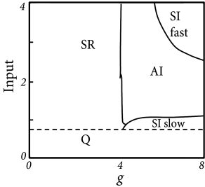
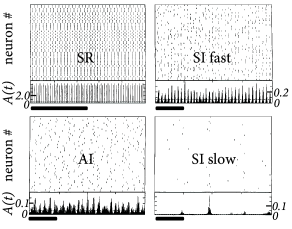
• Asynchronous irregular (AI):
• Synchronous regular (SR):
• Synchronous irregular (SI):

Networks of Nonlinear Integrate-and-Fire Neurons

Now we determine, for arbitrary nonlinear integrate-and-fire models driven by a diffusive input with constant mean \(\mu=RI_0\) and noise \(\sigma^{2}\), the distribution of membrane potentials \(p_0(u)\) as well as the linear response of the population activity \[ A(t)=A_0+A_1(t)=A_0+\int_{0}^{\infty} G(s)I_1(t-s) \mathrm{d}s, \tag{13.37} \] to a drive \(\mu(t)=R[I_0+I_1(t)]\).

Steady state population activity

We start with the continuity equation (13.7) \[ \frac{\partial }{\partial t}p(u,t)=-\frac{\partial }{\partial u}J(u,t)+A(t)\delta(u-u_r)-A(t)\delta(u-\theta_{reset}). \tag{13.38} \] In the stationary state, \[ \frac{\partial }{\partial u}J(u,t)=A(t)\delta(u-u_r)-A(t)\delta(u-\theta_{reset}). \tag{13.39} \]

The flux takes a constant value except at \(\theta_{reset}\) and \(u_r\). For \(u_r<u<\theta_{reset}\) the constant value \(J(u,t)=c>0\).

In the diffusion limit the flux according to (13.21) is \[ J(u,t)=\frac{1}{\tau_m} \left[f(u)+\mu(t)-\frac{1}{2}\sigma^{2}(t)\frac{\partial }{\partial u}\right]p(u,t). \tag{13.40} \]

In the stationary state, \(p(u,t)=p_0(u)\) and \(J(u,t)=c\) for \(u_r<u<\theta_{reset}\). Hence \[ \frac{\mathrm{d}p_0(u)}{\mathrm{d}u}=\frac{2\tau_m}{\sigma^{2}}\left[ \frac{f(u)+\mu}{\tau_m}p_0(u)-c\right]. \tag{13.41} \]

With initial condition \(p_0(\theta_{reset})=0\) and \(\mathrm{d} p_0/\mathrm{d}u |_{\theta_{reset}}=-2c\tau_m/\sigma^{2}\), one can integrate (13.41) from \(u=\theta_{reset}\). When the integration passes \(u=u_r\) the constant switches from \(c\) to \(0\). The integration is stopped at a lower bound \(u_{low}\) when \(p_0\) has approached \(0\).

Response to modulated input

Recall the exponential integrate-and-fire model \[ \tau \frac{\mathrm{d}}{\mathrm{d}t}u=-(u-u_{r})+\Delta_{T}\exp \left(\frac{u-\theta_{rh}}{\Delta_{T}}\right)+\mu, \tag{13.42} \]

We now add a small periodic perturbation to the input \[ I(t)=I_0+\varepsilon \cos (\omega t), \tag{13.43} \] where \(\omega=2\pi/T\). We expect the periodic drive to lead to a small periodic change in the population activity \[ A(t)=A_0+A_1(\omega)\cos (\omega t+\phi_{A}(\omega)). \tag{13.44} \]

We are to calculate \(\hat{G}\) that characterize the linear response or 'gain' at frequency \(\omega\) \[ \hat{G}(\omega)=\frac{A_1(\omega)}{\varepsilon}\mathrm{e}^{i \phi_{A}(\omega)} . \tag{13.45} \]

The small periodic drive at frequency \(\omega\) leads to a small periodic change in \(p(u,t)\) \[ p(u,t)=p_0(u)+p_1(u)\cos (\omega t +\phi_{p}(u)) \tag{13.48} \] We assume that \(\varepsilon\) is small so that \(p_1(u)\ll p_0(u)\) for most values of \(u\). We say that the change is at most of 'order \(\varepsilon\)'.

\(J(u,t)\) will also exhibit a small perturbation of order \(\varepsilon\). For (13.42) with \(u_{r}=0\) the flux is \[ J(u,t)=\left[ \frac{-u+RI(t)}{\tau_m}+\frac{\Delta_{T}}{\tau_m}\exp \left(\frac{u-\theta_{rh}}{\Delta_{T}}\right)-\frac{\sigma^{2}(t)}{2\tau_m}\frac{\partial }{\partial u}\right]p(u,t)=Q(u,t)p(u,t), \] (13.49)

The stationary state under the assumption of constant input \(I(t)=I_0\) has a flux \(J_0(u)=Q_0(u)p_0(u)\). In the presence of the periodic perturbation, the flux is \[ J(u,t)=J_0(u)+J_1(u)\cos (\omega t+\phi_{J}(u)) \tag{13.50} \]

with \[ J_1(u)\cos (\omega t+\phi_{J}(u))=Q_0(u)p_1(u)\cos (\omega t+\phi_{p}(u))+Q_1(u,t)p_0(u)+O(\varepsilon^{2}), \] (13.51)

where \(Q_1(u,t)=\varepsilon R\cos (\omega t)/\tau_m\) is the change of the operator \(Q\) to order \(\varepsilon\).

Note that the flux through the threshold \(\theta_{reset}\) gives the periodic modulation of the population activity.

We insert \(A,p,J\) into (13.38), include the phase into the definition of \(A_1,p_1(u),J_1(u)\), e.g. \(\hat{A}_1=A_1 \exp (i\phi_{A})\); the hat indicates the complex number. If we take the Fourier transform over time, (13.38) becomes \[ -\frac{\partial }{\partial u}\hat{J_1}(u)=i \omega \hat{p_1}(u)+\hat{A_1}[\delta(u-\theta_{reset})-\delta(u-u_r)]. \tag{13.52} \]

• We have quite arbitrarily normalized the membrane potential density to an integral of unity.
• The flux \(J_1\) in (13.51) can be quite naturally separated into two components. The first contribution to the flux is proportional to the perturbation \(p_1\) of the membrane potential density. The second component is caused by the direct action of the external current \(Q_1(u,t)=\varepsilon R\cos (\omega t)/\tau_m\).
• The explicit expression for \(Q_0\) and \(Q_1\) can be inserted into (13.51) \[ \frac{\partial }{\partial u} \hat{p_1}(u)=\frac{2}{\sigma^{2}}\left[ -u+RI_0+\Delta_{T}\exp \left(\frac{u-\theta_{rh}}{\Delta_{T}}\right)\right]\hat{p_1}(u)+\frac{2R \varepsilon}{\sigma^{2}}p_0(u)-\frac{2\tau}{\sigma^{2}}\hat{J_1}(u). \] (13.53)

We therefore have two first-order differential equations (13.52) and (13.53) which are coupled to each other.

(13.52) and (13.53) are two first-order differential equations which are coupled to each other. We drop the hats on \(J_1\), \(p_1\), \(A_1\) to lighten the notation. \(\varepsilon\) and \(A_1\) are parameters.

• We find the 'free' component by integrating (13.53) with \(\varepsilon=0\) in parallel with (13.52) with \(A_1=1\). The integration starts at the initial condition \(p_1(\theta_{reset})=0\) and \(J_1^{free}(\theta_{reset})=A_1=1\) and continues toward decreasing voltage values. Integration stops ar a lower bound \(u_{low}\) which we place at an arbitrary large negative value.
• We find the 'driven' component by integrating (13.53) with \(\varepsilon>0\) in parallel with (13.52) with parameter \(A_1=0\) starting at the initial condition \(p_1(\theta_{reset})=0\) and \(J_1^{\varepsilon}(\theta_{reset})=A_1=0\) and continue toward decreasing voltage values. Integration stops ar a lower bound \(u_{low}\)

Then we combinate them \[ J_1(u)=a_1 J_1^{free}(u)+a_2 J_1^{\varepsilon}(u) \] and \[ p_1(u)=a_1 p_1^{free}(u)+a_2 p_1^{\varepsilon}(u) \] We require a boundary condition \[ 0=J(u_{low})=a_1J_1^{free}(u_{low})+a_2 J_1^{\varepsilon}(u_{low}). \tag{13.54} \]

Recall that \(J_1^{\varepsilon}\) is proportional to the drive \(\varepsilon\). The factor \(a_1\) is the population response.

The gain factor is \[ \hat{G}(\omega)=\frac{A_1}{\varepsilon}=\frac{a_1}{\varepsilon}=-\frac{a_2}{\varepsilon}\frac{J_1^{\varepsilon}(u_{low})}{J_1^{free}(u_{low})}. \tag{13.55} \] which has an amplitude $() $ and a phase \(\phi_{G}\).

Neuronal adaptation and synaptic conductance

Adaptation currents

Suppose that the stochastic spike arrival can be modeled by a mean \(\mu(t)=R\langle I(t)\rangle\) plus a white-noise term \(\xi\). \[ \tau_m \frac{\mathrm{d}u}{\mathrm{d}t}=-(u-u_{rest})+\Delta_{T}\exp \left(\frac{u-\theta_{rh}}{\Delta _{T}}\right)-Rw+\mu(t)+\xi(t) \tag{13.59} \] \[ \tau_w \frac{\mathrm{d}w}{\mathrm{d}t}=a(u-u_{rest})-w+b\tau_w \sum_{t^{(f)}}^{} \delta(t-t^{(f)}). \tag{13.60} \]

Suppose furthermore that the time constant \(\tau_w\) of the adaptation variable \(w\) is larger than \(\tau_m\) and \(b\ll 1\) so the fluctuations of the adaptation variable \(w\) around $w $ are small. Therefore for the solution of the membrane potential density equations \(p_0(u)\) the adaptation variable can be approximated by a constant $w_0=w $.

Embedding in a network

The mean input \(\mu(t)\) to neuron \(i\) arriving at time \(t\) from population \(k\) is proportional to its activity \(A_k(t)\). The contribution of population \(k\) to the variance \(\sigma^{2}\) of \(\mu(t)\) is also proportional to \(A_k(t)\); cd. Eq.(13.31).

We can analyze the stationary states and their stability in a network of adaptive model neurons as

---

13.6 Neuronal adaptation and synaptic conductance https://neuronaldynamics.epfl.ch/online/Ch13.S6.html#Ch13.E61

---

Conductance input vs. current input

Synaptic input is more accurately described as a change in conductance \(g(t-t_j^{(f)})\), rather than as current injection. A time dependent synaptic conductance leads to a total synaptic current into neuron \(i\)
\[ I_i(t)=\sum_{j}^{} \sum_{f}^{} w_{ij}g_{ij}(t-t_j^{(f)})(u_i(t)-E_{syn}), \tag{13.63} \]

We will now show that, in the state of stationary asynchronous activity, conductance-based input can be approximated by an effective current input. The main effect of conductance-based input is that the membrane time constant of the stochastically driven neuron is shorter than the 'raw' passive membrane time constant.

We consider \(N_{E}\) excitatory and \(N_{I}\) inhibitory LIF neurons in the subthreshold regime \[ C \frac{\mathrm{d}u}{\mathrm{d}t}=-g_{L}(u-E_{L})-g_{E}(t)(u-E_{E})-g_{I}(t)(u-E_{I}), \tag{13.64} \] where \(C\) is the membrane capacity, \(g_{L}\) the leak conductance and \(E_{L}\), \(E_{E}\),\(E_{I}\) are the reversal potentials for leak, excitation, and inhibition, respectively. Input spikes at excitatory synapse lead to an increased conductance \[ g_{E}(t)=\Delta g_{E}\sum_{j}^{} \sum_{f}^{} \exp [-(t-t_j^{(f)})/\tau_{E}] \mathscr{H}(t-t_j^{(f)}). \tag{13.65} \]

The sum over \(j\) runs over all excitatory synapses. We assume that excitatory and inhibitory input spikes arrive with a total rate \(\nu_{E}\) and \(\nu_{I}\).

Using the methods from Chapter 8, we can calculate the mean excitatory conductance \[ g_{E,0}=\Delta g_{E}\nu_{E}\tau_{E}, \tag{13.66} \] where \(\nu_{E}\) is the total spike arrival rate at excitatory synapses.

The variance of the conductance is \[ \sigma_{E}^{2}=\frac{1}{2}(\Delta g_{E})^{2}\nu_{E} \tau_{E}. \tag{13.67} \]

Write the conductance as the mean plus a fluctuating component \[ g_{E,f}(t)=g_{E}(t)-g_{E,0}. \] This turns (13.64) into \[ C\frac{\mathrm{d}u}{\mathrm{d}t}=-g_0(u-\mu)-g_{E,f}(t)(u-E_{E})-g_{I,f}(t)(u-E_{I}), \tag{13.68} \] with a total conductance \(g_0=g_{L}+g_{E,0}+g_{I,0}\) and an input-dependent equilibrium potential \[ \mu=\frac{g_{L}E_{L}+g_{E,0}E_{E}+g_{I,0}E_{I}}{g_0}. \tag{13.69} \]

In (13.64) the dynamics is characterized by a raw membrane time constant \(C/g_{L}\) whereas (13.68) is controlled by an effective membrane time constant \[ \tau_{eff}=\frac{C}{g_0}= \frac{C}{g_{L}+g_{E,0}+g_{I,0}}, \tag{13.70} \]

and a mean depolarization \(\mu\) which acts as an effective equilibrium potential.

Then, we compare the momentary voltage \(u(t)\) with the effective equilibrium potential \(\mu\). The fluctuating part of the conductance in (13.68) can be written as \[ g_{E,f}(t)(u-E_{E})=g_{E,f}(t)(\mu-E_{E})+g_{E,f}(t)(u-\mu), \tag{13.71} \]

The second term on the RHS of (13.71) is small compared to the first term and needs to be dropped to arrive at a consistent diffusion approximation. The first term on the RHS of (13.71) can be interpreted as the summed effects of postsynaptic current pulses.

Colored Noise

Some synapse types, such as the NMDA component of excitatory synapses, are rather slow. A spike that has arrived at an NMDA synapse at time \(t_0\) generates a fluctuation, which cause the input to exhibit temporal correlations.

We have two approaches to colored noise in the membrane potential density equations.

The first approach is to approximate colored noise by white noise and replace the temporal smoothing by a broad distribution of delays. Problem set: current-based. The mean input to a neuron \(i\) in population \(n\) arising from other populations \(k\) is \[ I_i(t)=\sum_{k}^{} C_{nk}w_{nk}\int_{0}^{\infty} \alpha_{nk}(s)A(t-s) \mathrm{d}s, \tag{13.72} \]

Suppose \(C_{nk}\) is a large number, but the population \(k\) itself is larger so that the connectivity \(C_{nk}/N_k \ll 1\). We now replace \(\alpha(s)\) by \(q \delta(s-\Delta)\) such that \(q=\int_{0}^{\infty} \alpha(s) \mathrm{d}s\). For each of the \(C_{nk}\) connections we randomly draw the transmission delay \(\Delta\) from a distribution \(p(\Delta)=\alpha(\Delta)/q\). Because of the low connectivity, we may assume that the firing of different neurons is uncorrelated. The broad distribution of delays stabilizes the stationary state of asynchronous firing.

The second approach consists in an explicit model of the synaptic current variables. We focus on a single population coupled to itself and suppose that the synaptic current pulses are exponential \(\alpha(s)=(q/\tau_q)\exp (-s/\tau_q)\). The driving current of a neuron \(i\) in a population \(n\) is then \[ \frac{\mathrm{d}I_i}{\mathrm{d}t}=-\frac{I_i}{\tau_q}+C_{nn}w_{nn}\frac{q}{\tau_q}A_n(t) \tag{13.73} \] which we can verify by taking the temporal derivative of (13.72). \(A(t)\) has a mean \(\mu(t)\) (which is the same for all neurons) and a fluctuating part \(\xi_{i}(t)\) with white-noise characteristics: \[ \frac{\mathrm{d}I_i}{\mathrm{d}t}=-\frac{I_i}{\tau_q}+\mu(t)+\xi_{i}(t). \tag{13.74} \] (13.74) needs to be combined with the differential equation for the voltage \[ \tau_m \frac{\mathrm{d}u_i}{\mathrm{d}t}=f(u_i)+RI_{i}(t), \tag{13.75} \] We now have two coupled differential equations, the momentary state of a population of \(N\) neurons is described by a two-dimensional density \(p(u,I)\).

We recall that, in the case of white noise, the membrane potential density at threshold vanishes. The main insight for the mathematical treatment of the membrane potential density equations in two dimensions is that the density at threshold \(p(\theta_{reset},I(t))\) is finite, whenever the momentary slope of the voltage \(\mathrm{d}u/\mathrm{d}t \propto RI(t)+f(\theta_{reset})\) is positive.

Summary

The momentary state of a population of one-dimensional integrate-and-and fire neurons can be characterized by the membrane potential density \(p(u,t)\). The continuity equation describes the evolution of \(p(u,t)\) over time. In the special case that neurons in the population receive many inputs that each cause a small change of the membrane potential, the continuity equation has the form of a Fokker-Planck equation. Several populations of integrate-and-fire neurons interact via the population activity \(A(t)\) which is identified with the flux across the threshold.

The stationary state of the Fokker-Planck equation and the stability of the stationary solution can be calculated by a mix of analytical and numerical methods, be it for a population of independent or interconnected neurons. The mathematical and numerical methods developed for membrane potential density equations apply to leaky as well as to arbitrary nonlinear one-dimensional integrate-and-fire model. A slow adaptation variable such as in the adaptive exponential integrate-and-fire model can be treated as quasi-stationary in the proximity of the stationary solution. Conductance input can be approximated by an equivalent current-based model.