Neuronal Dynamics (9)
Noisy Output: Escape Rate and Soft Threshold
The online version of this chapter:
Chapter 9 Noisy Output: Escape Rate and Soft Threshold https://neuronaldynamics.epfl.ch/online/Ch9.html
Escape noise
In this section the notion of escape noise is introduced.
Escape rate
\(\theta\): formal threshold
In Ch6, the value of the membrane potential of a SRM can be expressed as \[ u(t)=\sum_{f}^{} \eta(t-t^{(f)})+\int_{0}^{\infty} \kappa(s)I^{det}(t-s) \mathrm{d}s +u_{rest}, \tag{9.1} \]
where \(I^{det}\) is the known driving current and \(\kappa\) and \(\eta\) are filters that describe the response of the membrane to an incoming pulse or an outgoing spike.
Replace the strict threshold by a stochastic firing criterion. In the noisy threshold model, spikes can occur at any time with a probability density \[ \rho(t)=f(u(t)-\theta), \tag{9.2} \]
In the mathematical theory of point processes, the quantity \(\rho\) is called a 'stochastic intensity'. We refer to \(\rho\) as a firing intensity.
A common choice for \(f\) is the exponential, \[ f(u-\theta)=\frac{1}{\tau_0}\exp [\beta(u_0-\theta)] \tag{9.3} \] where \(\beta\) and \(\tau_0\) are parameters. For \(\beta \to \infty\), the soft threshold turns into a sharp one.
More generally, the spike trigger process could also depend on the slope \(\dot{u}=\mathrm{d}u/\mathrm{d}t\). \[ \rho(t)=f[u(t)-\theta,\dot{u}]. \tag{9.4} \]
Transition from continuous time to discrete time
We consider the probability \(P_{F}(u)\) of firing in a finite time step given the neurons has membrane potential \(u\).
In a straightforward discretization scheme, \(\int_{t}^{t+\Delta t} \rho(t') \mathrm{d}t'\thickapprox \rho(t)\Delta t\). \(\Delta t\) must be taken extremely short so as to guarantee \(\rho(t)\Delta t<1\).
In an improved discretization scheme, \[ P_{F}(u)=\operatorname{Pr}\{\text{spike in} \ [t,t+\Delta t]|u(t)\}\thickapprox 1-\exp \{-\Delta t f[u(t)-\theta] \}. \] (9.8)
For small \(\Delta t\), the probability \(P_{F}\) scales as \(f \Delta t\).
For an exponential escape rate, an increase in the discretization \(\Delta t\) mainly shifts the firing curve to the left.
Likelihood of a spike train
In this section we determine the likelihood that a specific spike train is generated by a neuron model with escape noise.
Assume a spike train which is generated by an escape noise process
\[ \rho(t)=f(u(t)-\theta) \tag{9.9} \]
and the membrane potential \(u(t)\) arises from the dynamics of one of the dynamics of one of the generalized integrate-and-fire models such as the SRM.
The likelihood \(L^{n}\) that spikes occur at the times \(t^{(1)},\cdots ,t^{(f)},\cdots ,t^{(n)}\) is \[ L^{n}(\{t^{(1)},t^{(2)},\cdots ,t^{(n)}\})=\rho(t^{(1)})\cdot \rho(t^{(2)})\cdots \rho(t^{(n)}) \exp \left[ -\int_{0}^{T} \rho(s) \mathrm{d}s\right], \tag{9.10} \] where \([0,T]\) is the observation interval. The product on the right-hand side contains the momentary firing intensity \(\rho(t^{(f)})\) at the firing times \(t^{(1)},t^{(2)},\cdots ,t^{(n)}\). The exponential factor takes into account that the neuron needs to 'survive' without firing in the intervals between the spikes.
Actually, \[ \begin{aligned} L^{n}(\{t^{(1)},t^{(2)},\cdots ,t^{(n)}\})= \exp \left[-\int_{0}^{t^{(1)}} \rho(s) \mathrm{d}s\right]\cdot \\ \rho(t^{(1)})\exp \left[-\int_{t^{(1)}}^{t^{(2)}} \rho(s) \mathrm{d}s\right]\cdot \ldots\\ \rho(t^{(n)})\exp \left[-\int_{t^{(n)}}^{T} \rho(s) \mathrm{d}s\right]. \end{aligned} \] (9.11)
Sometimes it is more convenient to work with the logarithm of the likelihood, called the log-likelihood \[ \log L^{n}(\{t^{(1)},\cdots ,t_i^{(f)},t^{(n)}\})=-\int_{0}^{T} \rho(s) \mathrm{d}s+\sum_{f=1}^{n} \log \rho(t_i^{(f)}). \tag{9.12} \]
Example: Discrete-time version of likelihood and generative model
For a discrete-time simulation, the probability of finding an empty time bin (spike count \(n_t=0\)) is \[ \operatorname{Pr} \{\text{silent in} \ [t,t+\Delta t]\}=1-P_{t}=\exp \{-\Delta t \rho(t)\} \tag{9.13} \]
With sufficiently small \(\Delta t\), it is impossible to have two spikes in a time bin \(\Delta t\). This reflects the fact that, because of neuronal refractoriness, neurons cannot emit two spikes in a time bin shorter than, say, half the duration of an action potential.
\[ P_{total}=\prod_{bins \ with \ spike}^{} [P_t] \cdot \prod_{empty \ bins}^{} [1-P_t]=\prod_{t}^{} \{[P_t]^{n_t}\cdot [1-P_t]^{1-n_t}\}, \] where the product runs over all time bins and \(n_t \in \{0,1\}\) is the spike count number in each bin.
The observed spike trains has \[ P_{total}=\prod_{k=1}^{n} [P_{t_k}]\cdot \prod_{k'}^{} [1-P_{t_{k'}}]. \tag{9.16} \]
All time bins that fall into the interval between two spikes can be regrouped as follows \[ \prod_{\{k'|t_k<t_{k'}<t_{k+1}\}}^{}[1-P_{t_{k'}}]\exp \{-\Delta t \rho(t_{k'})\}=\exp \left\{-\sum_{t_k<t_{k'}<t_{k+1}}^{} \Delta t \rho(t_{k'})\right\}. \] (9.17)
The Riemann-sum on the right-hand side of (9.17) then turns into an integral. Combine the limit in (9.16), we have \[ P_{total}=L^{n}(\{t^{(1)},t^{(2)},\cdots ,t^{(n)}\})(\Delta t)^{n}, \tag{9.18} \]
Renewal Approximation of the Spike Response Model
In this section we apply the escape noise formalism to the SRM and show an interesting link to the renewal statistics encountered in Ch7.
We focus a SRM with escape noise. If the firing rate is low, so that the interspike interval is much longer than the decay time of the refractory kernel \(\eta\), then we can truncate the sum over past firing times and keep track only of the effect of the most recent spike \[ u(t)=\eta(t-\hat{t})+\int_{0}^{\infty} \kappa(s)I^{det}(t-s) \mathrm{d}s +u_{rest}, \tag{9.19} \] where \(\hat{t}\) denotes the last firing time \(t^{(f)}<t\).
(9.19) is called the 'short-term momory' approximation of the SRM and abbreviated as SRM\(_0\). Sometimes we write \(u(t|\hat{t})\) intstead of \(u(t)\) to emphasize that the value of the membrane potential depends only on the most recent spike.
Input potential: \[ h(t)=\int_{0}^{\infty} \kappa(s)I^{det}(t-s) \mathrm{d}s \tag{9.20} \] which allows us to rewrite (9.19) as \[ u(t|\hat{t})=\eta(t-\hat{t})+h(t)+u_{rest}. \tag{9.21} \]
The escape rate \[ \rho(t|\hat{t})=f(u(t|\hat{t})) \tag{9.22} \] depends on the time since the last spike and, implicitly, on the stimulating current \(I^{det}(t)\). Given the last spike time \(\hat{t}\) and the input \(I^{det}(t')\) for \(t'<t\), we can calculate the probability density that the next spike occurs at time \(t>\hat{t}\) \[ P_{I}(t|\hat{t})=\rho(t|\hat{t})\exp \left[-\int_{\hat{t}}^{t} \rho(t'|\hat{t}) \mathrm{d}t'\right]. \tag{9.23} \]
Example: Interval distribution with exponential escape noise
We study a model SRM\(_0\) with membrane potential \(u(t|\hat{t})=\eta(t-\hat{t})+h(t)\) and choose a refractory kernel with absolute and relative refractoriness defined as \[ \eta(s)= \begin{cases} -\infty, s<\Delta^{abs} \\ -\eta_0 \exp \left(-\frac{s-\Delta^{abs}}{\tau}\right), s>\Delta^{abs} \end{cases} \] (9.24)
and the exponential escape rate (9.3).
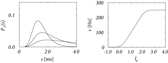
The above figure shows the interval distribution for constant input current \(I_0\) as a function of \(s=t-\hat{t}\). With the normalization \(\int_{0}^{\infty} \kappa(s) \mathrm{d}s=1\), we have \(h_0=I_0\). The gain function \(\nu=g(I_0)\) of a noisy SRM\(_0\) neuron is shown on the right.
We now study the same model with periodic input \(I^{det}(t)=I_0+I_1 \cos (\Omega t)\). This leads to an input potential \(h(t)=h_0+h_1 \cos (\Omega t+\varphi_1)\) with bias \(h_0=I_0\) and a periodic component with a certain amplitude \(h_1\) and phase \(\varphi_1\).
The result of \(P_{I}(t|0)\) is shown in the following figure on the left.


The periodic component of the input is well represented in the response of the neuron. This example illustrates how neurons in the auditory system can transmit stimuli of frequencies higher than the mean firing rate of the neuron.
From noisy inputs to escape noise
Sometimes without noise there would be no output spike. On the other hand, at very high noise levels, the modulation of the interval distribution would be much weaker. Thus a certain amount of noise is beneficial for signal transmission.
In this section we show that the noisy, unknown part \(\xi(t)\) in the input can be approximated by an appropriately chosen escape function.
Example: Adaptive exponential integrate-and-fire model with noisy input
Suppose that the AdEx model is driven by an input as \(I(t)=I^{det}(t)+\xi(t)\) containing a ripidly moving deterministic signal \(I^{det}(t)\) as well as a white noise component \(\xi(t)\).
We approximate the voltage of the AdEx model by a linear model \[ u(t)=\sum_{f}^{} \eta(t-t_i^{(f)})+\int_{0}^{\infty} \kappa(s)I^{det}(t-s) \mathrm{d}s+u_{rest}. \tag{9.26} \]
In the subthreshold regime \(u<\theta-\Delta_{T}\), the filters \(\kappa\) and \(\eta\) can be calculated analytically. (9.26) combined with the exponential escape rate \[ f(u-\theta)=\frac{1}{\tau_0}\exp [\beta(u-\theta)] \]
describes the activity of the AdEx with noisy input surprisingly well. In the presence of an input noise \(\xi(t)\) the exponential term in the voltage equation of the AdEx model can be replaced by an exponential escape rate.
Leaky integrate-and-fire model with noisy input
Though the probability density at \(u=\theta\) vanishes in the presence of threshold, we can approximate the probability density near \(u=\theta\) by the 'free' distribution (i.e., without the threshold) \[ \operatorname{Pr} \{u \ \text{reaches} \ \theta \ \text{in} \ [t,t+\Delta t]\}\propto \Delta t \exp \left\{-\frac{[u_0(t)-\theta]^{2}}{2\langle \Delta u^{2}(t)\rangle}\right\} \tag{9.28} \]
那么Fig 9.10是什么意思呢?\([t,t+\Delta t]\) 间达到threshold的概率为什么与右边成正比呢
We can replace the time dependent variance \(2\langle \Delta u(t)^{2}\rangle\) by its stationary value \(\sigma^{2}\)(see (8.13)). So \[ f(u_0-\theta)=\frac{c_1}{\tau_m}\exp \left\{-\frac{[u_0(t)-\theta]^{2}}{\sigma^{2}}\right\} \tag{9.29} \] (Arrhenius formula)
\(c_1/\tau_m\) shows that the escape rate has units of one over time.
If at \(t=t_0\), an input current pulse causes a jump of the membrane trajectory by amount \(\Delta u>0\), then there is a nonzero probability that the neuron fires exactly at \(t_0\). We expect an increase of the instantaneous rate proportional to \(\dot{u}_{0}\), so we study \[ f(u_0,\dot{u}_0)=\left(\frac{c_1}{\tau_m}+\frac{c_2}{\sigma}[\dot{u}_0]_{+}\right)\exp \left\{-\frac{[u_0(t)-\theta]^{2}}{\sigma^{2}}\right\}, \tag{9.30} \] where \([x]_{+}=x\) for \(x>0\) and zero otherwise. We call (9.30) he Arrhenius&Current model.
(9.30) depends only on the dimensionless variable \[ x(t)=\frac{u_0(t)-\theta}{\sigma}, \tag{9.31} \]
and its derivative \(\dot{x}\). A distance of \(u-\theta=-10 mV\) at high noise (e.g., \(\sigma=10 mV\)) is as effective in firing a cell as a distance of \(1mV\) at low noise (\(\sigma=1mV\)).
Example: Comparison of diffusion model and Arrhenius&Current escape rate
The interval distribution for the diffusive white noise model (derived from stochastic spike arrival) and that for the Arrhenius&Current escape model yields an excellent approximation to the diffusive noise model.
An obvious shortcoming of (9.30) is that the instantaneous rate decreases with \(u\) for \(u>\theta\). The superthreshold behavior can be corrected if we replace the Gaussian \(\exp (-x^{2})\) by \(2\exp(-x^{2})/[1+\text{erf}(-x)]\). The subthreshold behavior remains unchanged compared to (9.30) but the superthreshold behavior of the escape rate \(f\) becomes linear.
Stochastic resonance
Existence of an optimum for the noise amplitude which has motivated the name stochastic resonance is a counterintuitive phenomenon.
In the absence of noise, a subthreshold stimulus \(I(t)\) does not generate action potentials so that no information on the temporal structure of the stimulus can be transmitted. On the other hand, for very large noise \(\sigma \to \infty\), spike firing occurs at a constant rate, irrespective of the temporal structure of the input.
Even though stochastic resonance does not require periodicity, it is typically studied with a periodic input signal \[ I^{det}(t)=I_0+I_1\cos (\Omega t). \tag{9.32} \] For \(t-\hat{t}\gg\tau_m\), the membrane potential of the noise-free reference trajectory has the form \[ u_0(t)=u_{\infty}+u_1 \cos (\Omega t+\varphi_1), \tag{9.33} \] where \(u_1\) and \(\varphi_1\) are amplitude and phase of its periodic component. We compute the signal-to-noise ratio (SNR).
The signal \(\mathscr{S}\) is measured as the amplitude of the power spectral density of the spike train evaluated at frequency \(\Omega\), i.e., \(\mathscr{S}=\mathscr{P}(\Omega)\). The noise level \(\mathscr{N}\) is usually estimated from the noise power \(\mathscr{P}_{Poisson}\) with the same number of spikes as the measured spike train.
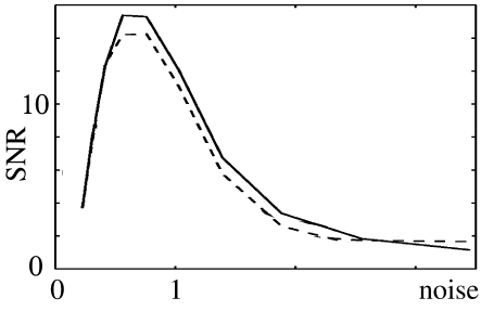
The above figure shows the SNR \(\mathscr{S}/\mathscr{N}\) of a periodically stimulated integrate-and-fire neuron as a function of the noise level \(\sigma\). They exhibit a peak at \[ \sigma^{opt}\thickapprox \frac{2}{3}(\theta-u_{\infty}) \tag{9.34} \]
accordingly, \[ 2\sqrt{\langle \Delta u^{2}\rangle}\thickapprox \theta-u_{\infty}. \tag{9.35} \]
Example: Extracting oscillations
We study the question whether an integrate-and-fire neuron or a SRM neuron is only sensitive to the total number of spikes that arrive in some time window \(T\), or also to the relative timing of the input spikes.
We compare two different scenarios of stimulation. In the first scenario input spikes arrive with a periodically modulated rate, \[ \nu^{in}(t)=\nu_0+\nu_1 \cos (\Omega t) \tag{9.36} \] with \(0<\nu_1<\nu_0\). Spikes are generated by this inhomogeneous Poisson process.
In the second scenario input spikes are generated by a homogeneous Poisson process with constant rate \(\nu_0\).
In a large interval \(T\gg\Omega ^{-1}\), we expect in both cases a total number of \(\nu_0T\) input spikes.
It is found that the spike count numbers \(n^{(1)}\) and \(n^{(2)}\) are significantly different if the threshold is in the range \[ u_{\infty}+\sqrt{\langle \Delta u^{2}\rangle}<\theta<u_{\infty}+3\sqrt{\langle \Delta u^{2}\rangle} \tag{9.37} \]
This means that a neuron in the subthreshold regime is capable of transforming a temporal code (amplitude \(\nu_1\) of the variations in the input) into a spike count code.