Neuronal Dynamics (6)
Adaptation and Firing Patterns
The online version of this chapter:
Chapter 6 Adaptation and Firing Patterns https://neuronaldynamics.epfl.ch/online/Ch6.html
Adaptive Exponential Integrate-and-Fire
A single equation is not sufficient to describe the variety of firing patterns that neurons exhibit in response to a step current. We couple the voltage equation to abstract current variables \(w_k\). The set of equation is \[ \tau_m \frac{\mathrm{d}u}{\mathrm{d}t}=f(u)-R \sum_{k}^{} w_k+RI(t) \] (6.1) \[ \tau_k \frac{\mathrm{d}w_k}{\mathrm{d}t}=a_k(u-u_{rest})-w_k+b_k\tau_k\sum_{t^{(f)}}^{} \delta(t-t^{(f)}). \] (6.2)
the adaptation current is fed back to the voltage equation with resistance \(R\). The voltage variable \(u\) is reset if the membrane potential reaches the numerical threshold \(\Theta_{reset}\). The moment \(u(t)=\Theta_{reset}\) defines the firing time \(t^{(f)}=t\). After firing, integration of the voltage restarts at \(u=u_r\). The parameters \(b_k\) are the 'jump' of the spike-triggered adaptation.
One possible biophysical interpretation of the increase is that during the action potential calcium enters into the cell so that the amplitude of a calcium-dependent potassium current is increased.
The adaptive Exponential Integrate-and-Fire model (AdEx) consists of an exponential nonlinearity in the voltage equation coupled to a single adaptation variable \(w\) \[ \tau_m \frac{\mathrm{d}u}{\mathrm{d}t}=-(u-u_{rest})+\Delta_{T} \exp \left(\frac{u-\theta_{rh}}{\Delta_{T}}\right)-Rw+RI(t) \] (6.3) \[ \tau_w \frac{\mathrm{d}w}{\mathrm{d}t}=a(u-u_{rest})-w+b\tau_w \sum_{t^{(f)}}^{} \delta(t-t^{(f)}). \] (6.4)
At each threshold crossing the voltage is reset to \(u=u_r\) and the adaptation variable \(w\) is increased by an amount \(b\). Adaptation is characterized by two parameters: \(a\) couples adaptation to the voltage and is the source of subthreshold adaptation. Spike-triggered adaptation is controlled by a combination of \(a\) and \(b\). The choice of \(a\) and \(b\) largely determines the firing patterns of the neuron and can be related to the dynamics of ion channels.
Example: Izhikevich model
This model uses the quadratic integrate-and-fire model for the first equation \[ \tau_m \frac{\mathrm{d}u}{\mathrm{d}t}=-(u-u_{rest})(u-\theta)-Rw+RI(t) \] \[ \tau_w \frac{\mathrm{d}w}{\mathrm{d}t}=a(u-u_{rest})-w+b\tau_w \sum_{t^{(f)}}^{} \delta(t-t^{(f)}). \]
If \(u=\theta_{reset}\), the voltage is reset to \(u=u_r\) and the adaptation variable \(w\) is increased by an amount \(b\). Normally \(b\) is positive, but \(b<0\) is also possible.
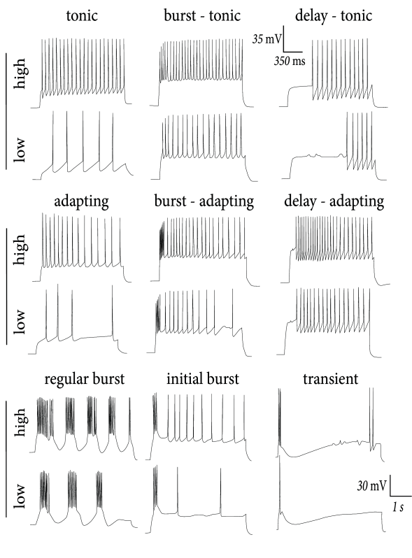 > Multiple firing patterns in
cortical neurons. For each type, the neuron is stimulated with a step
current with low or high amplitude.
> Multiple firing patterns in
cortical neurons. For each type, the neuron is stimulated with a step
current with low or high amplitude.
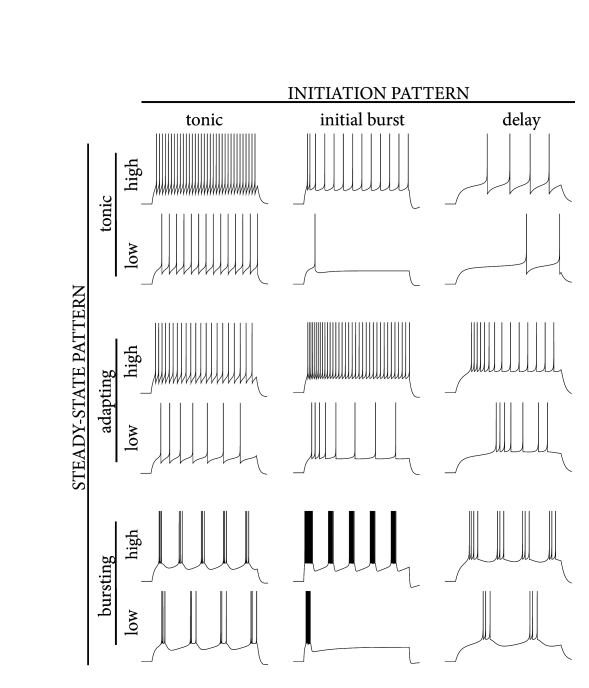 > Multiple firing patterns in
the AdEx neuron model. The spiking response can be classified by the
steady-state firing behavior (vertical axis: tonic, adapting, bursting)
and by its transient initiation pattern as shown along the horizontal
axis: tonic (i.e. no special transient behavior), initial burst, or
delayed spike initiation.
> Multiple firing patterns in
the AdEx neuron model. The spiking response can be classified by the
steady-state firing behavior (vertical axis: tonic, adapting, bursting)
and by its transient initiation pattern as shown along the horizontal
axis: tonic (i.e. no special transient behavior), initial burst, or
delayed spike initiation.
Example: Leaky model with adaptation
Adaptation variables \(w_k\) can also be combined with a standard leaky integrate-and-fire model \[ \tau_m \frac{\mathrm{d}u}{\mathrm{d}t}=-(u-u_{rest})-R\sum_{k}^{} w_k +RI(t) \] (6.7)
\[ \tau_k \frac{\mathrm{d}w_k}{\mathrm{d}t}=a(u-u_{rest})-w_k+b_k\tau_k \sum_{t^{(f)}}^{} \delta(t-t^{(f)}) \] (6.8)
At the moment of firing, defined by the threshold condition \(u(t^{(f)})=\theta_{reset}\), the voltage is reset to \(u=u_r\) and the adaptation variable \(w_k\) are increased by an amount \(b_k\).
Firing Patterns
Classification of Firing Patterns
It is advisable to separate the steady-state pattern from the initial transient phase. The initiation phase refers to the firing pattern right after the onset of the current step.
Three main initiation pattern: the initiation can not be distinguished from the rest of the spiking response (tonic); the neuron responds with a significantly greater spike frequency in the transient (initial burst) than in the steady state; the neuronal firing starts with a delay (delay).
Three main steady state patterns: regularly spaced spikes (tonic); gradually increasing interspike intervals (adapting); or regular alternations between short and long interspike intervals (bursting).
Irregular firing patterns are also possible in the AdEx model, but the discussion below is restricted to deterministic models.
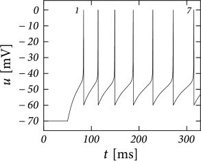
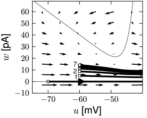
Example: Tonic, Adapting and Facilitating
When the subthreshold coupling \(a\) is small and the voltage reset is low (\(u_r \thickapprox u_{rest}\)), the AdEx response is either tonic or adapting. This depends on the jump \(b\) and the time scale \(\tau_w\).
A large jump with a small time scale creates evenly spaced spikes at low frequency.On the other hand, a small spike-triggered current decaying on a long timescale can accumulate strength over several spikes and therefore successively decreases the net driving current \(I-w\). In general, weak but long-lasting spike-triggered currents cause spike-frequency adadptation while short but strong currents lead to a prolongation of the refactory period. There is a continuum between purely tonic spiking and strongly adapting.
When the spike-triggered curent is depolarizing \((b<0)\) the interspike interval may gradually decreases, leading to spike-frequency facilitation.
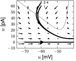
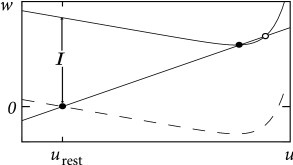
Phase plane analysis of non-linear integrate-and-fire models in two dimensions
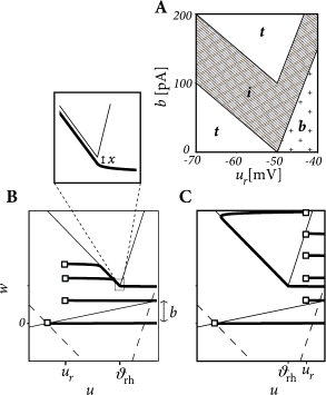
In the AdEx model, the \(u-\)nullcline is again linear in the subthreshold regime and rises exponentially when \(u\) is close to \(\theta\). Upon current injection, the \(u-\)nullcline is shifted vertically by an amount proportional to the magnitude of the current \(I\).
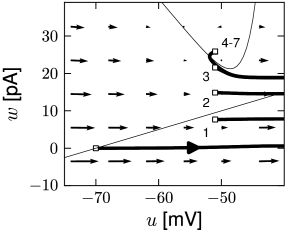
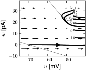
Each time the trajectory reaches \(u=\theta_{reset}\), it will be re-initialized at a reset value \((u_r,w+b)\).
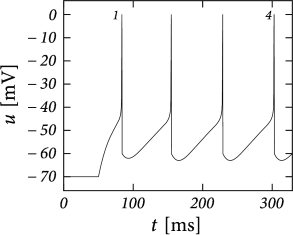
There are three regions of the phase plane with qualitatively different ensuing dynamics. A 'detour reset' corresponds to a downswing of the membrane potential after the end of the action potential. The distinction between detour and direct resets is helpful to understand how different firing patterns arise.
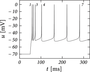
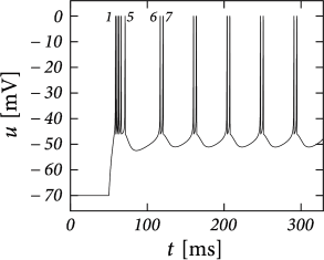
Example: Bursting
Initial burst: a neuron first fires a group of spikes at a considerably higher spiking frequency than the steady-state frequency.
The shape of the voltage trajectory after the end of the action potential (downswing or not) can be used to distinguish between adapting (strictly detour or strictly direct resets) and initial bursting (first direct then detour resets).
By alternation between direct and detour resets, regular bursting can arise.
AdEx can also produce an irregular alternation. The parameters for irregular firing occupies a small and patchy volume in parameter space.
Exploring the Space of Reset Parameters
Boundaries in the parameter space mark transitions between different types of firing pattern - which are often correlated with types of cells.
Apply a step current with an amplitude twice as large as the minimal current necessary to elicit a spike and study the dependence of the observed firing pattern on the reset parameter \(u_r\) and \(b\). All the other parameters are kept fixed.
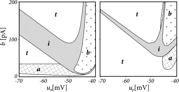
- The line separating initial bursting and tonic firing resembles the shape of the \(u-\)nullcline. That's because the \(u-\)nullcline plays an important role in determining whether the reset is 'direct' or leads to a 'detour'.
- Regular bursting is possible, if the voltage reset \(u_r\) is located above the voltage threshold \(\theta\). Irregular firing patterns are found within the bursting region of the parameter space.
- Adapting firing patterns occur only over a restricted range of jump amplitudes \(b\) of the spike-triggered adaptation current.
Example: Piecewise-Linear Model
Consider a piecewise linear version of the AdEx model \[ f(u)= \begin{cases} -(u-u_{rest}) \quad u\leqslant \theta_{rh} \\ \Delta_{T}(u-u_p) \quad \text{otherwise} \end{cases} \] (6.9)
with \[ u_p=\theta_{rh}+\frac{\theta_{rh}-u_{rest}}{\Delta_T}, \] (6.10) which we insert into the voltage equation \(\tau_m \mathrm{d}u/\mathrm{d}t=f(u)+RI-Rw\). Note that the \(u-\)nullcline is given by \(w=f(u)/R+I\) and takes at \(u=\theta_{rh}\) its minimum value \(w_{min}=f(\theta_{rh})/R+I\).
We assume separation of timescale (\(\tau_m/\tau_w \ll 1\)) and exploit the fact that the trajectories in the phase plane are nearly horizontal - unless they approach the \(u-\)nullcline.
Map the initial condition \((u_r,w_r)\) after a first reset to the value \(w_e\) of the adaptation variable at the end of the trajectory: \(w_e=M(u_r,w_r)\). The next reset starts then from \((u_r,w_e+b)\). All trajectories with \(w_r<w_{min}\) remain horizontal, so that \(w_e=w_r\).
If \(w_r>w_{min}\), we distinguish two possible cases. The first one corresponds to a voltage reset below the threshold, \(u_r<\theta_{rh}\). A trajectory initiated at \(u_r<\theta_{rh}\) evolves horizontally until it comes close to the left branch of the \(u-\)nullcline. It then follows the \(u-\)nullcline at a small distance \(x(u)\) below it. The distance can be shown to be \[ x(u)=\frac{\tau_m}{\tau_w}[I-(a+R^{-1})(u-u_{rest})], \] (6.11) which vanishes in the limit \(\tau_m/\tau_w \to 0\). For \(u_r<\theta_{rh}\). \[ M(u_r,w_r)= \begin{cases} w_r \quad w_r<f(u_r)/R+I \\ f(\theta_{rh})/R+I \quad \text{otherwise} \end{cases} \] (6.12) If \(u_r>\theta_{rh}\) then we have a direct reset (i.e.,movement starts to the right) if \((u_r,w_r)\) lands below the right branch of the \(u-\)nullcline and a detour reset otherwise \[ M(u_r,w_r)= \begin{cases} w_r \quad w_r<f(u_r)/R+I \\ f(\theta_{rh})/R+I \quad \text{otherwise} \end{cases} \] (6.13)
 > Fig.6.7
The map \(M\) uniquely defines the firing pattern. Regular bursting is possible only if \(u_r>\theta_{rh}\) and \(b<f(u_r)-f(\theta_{rh})\) so that at least one reset in each burst lands below the \(u-\)nullcline. For \(u_r>\theta_{rh}\), we have tonic spiking with detour resets when \(b>f(u_r)+I\) and initial bursting if \(f(u_r)+I>b>f(u_r)-f(\theta_{rh})+x(\theta_{rh})\).
If \(u_r\leqslant \theta\) we have tonic spiking with detour resets when \(b>f(u_r)+I\), tonic spiking with direct reset when \(b<f(u_r)-f(\theta_{rh})\) and initial bursting if \(f(u_r)+I>b>f(u_r)-f(\theta_{rh})\). Note that the rough layout of the parameter regions in Fig.6.7A.
Exploring the Space of Subthreshold Parameters
While the exponential integrate-and-fire model losses stability always via a saddle-node bifurcation, the AdEx can become unstable either via a Hopf or a saddle-node bifurcation.
In the AdEx, an eigenvalue analysis shows that the stable fixed point looses stability via a Hopf bifurcation if \(aR>\tau_m/\tau_w\).
Otherwise, when the coupling from voltage to adaptation (parameter \(a\)) and back from adaptation to voltage (parameter \(R\)) are both weak, an increase in the current causes the stable fixed point to merge with the unstable one, so that both disappear via a saddle-node bifurcation.
The type of bifurcation has no influence on the firing pattern (bursting, adapting, tonic) which depends mainly on the choice of reset parameters.
However, the subthreshold parameters do control the presence or absence of oscillations in response to a short current pulse.
resonator: a model showing damped oscillations.
integrator: a model without damped oscillations.
The presence of damped oscillations depends non-linearly on \(a/g_{L}\) and \(\tau_m/\tau_w\) as summarized in the figure below.
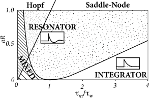
The frequency of the damped oscillation is given by \[ \omega=\frac{4}{\tau_w}\left[aR-\frac{2\tau_w}{\tau_m}\left(1-\frac{\tau_m}{\tau_w}\right)^{2}\right] \] (6.14)
Example: Transient Spiking
Upon the onset of a current step, some neurons may fire a small number of spikes and then remain silent, even if the stimulus is maintained for a very long time. An AdEx model with subthreshold coupling \(a>0\) can explain this phenomenon whereas pure spike-triggered adaptation (\(a=0;b>0\)) cannot account for it, because adaptation would eventually decay back to zero so that the neuron fires another spike.
Choose parameter \(a\) and \(\tau_w\) such that the neuron is in the resonator regime. The voltage response to a step input then exhibits damped oscillations. Phase plane analysis reveals that sometimes several resets are needed before the trajectory is attracted towards the fixed point.
Biophysical Origin of Adaptation
We now show that the variables \(w_k\) can be linked to the biophysics of ion channels and dendrites.
Subthreshold adaptation by a single slow channel
First our aim is to give a biophysical interpretation of the parameters \(a\), \(\tau_w\), and the variable \(w\) that show up in the adaptation equation \[ \tau_w \frac{\mathrm{d}w}{\mathrm{d}t}=a(u-E_0)-w. \] (6.15) Here and in the following we write \(E_0\) instead of \(u_{rest}\) in order to simplify notation and keep the treatment slightly more general.
We know rapid activation of the sodium channels, important during the upswing of action potentials, is well approximated by the exponential nonlinearity in the voltage equation of the AdEx model. We will see now that the subthreshold current \(w\) is linked to the dynamics of other ion channels with a slower dynamics.
Let us focus on the model of a membrane with a leak current and a single, slow, ion channel, say a potassium channel of the Hodgkin-Huxley type \[ \tau_m \frac{\mathrm{d}u}{\mathrm{d}t}=-(u-E_{L})-R_{L}g_{K}n^{p}(u-E_k)+R_{L}I_{ext} \] (6.16)
where \(R_{L}\) and \(E_{L}\) are the resistance and reversal potential of the leak current, \(\tau_m=R_{L}C\) the membrane time constant, \(g_{K}\) the maximal conductance of the open channel and \(n\) the gating variable (which appears with arbitrary power \(p\)) with dynamics \[ \frac{\mathrm{d}n}{\mathrm{d}t}=-\frac{n-n_0(u)}{\tau_n(u)}. \] (6.17)
As long as the membrane potential stays below threshold, we can linearize the equations (6.16) and (6.17) aroung the resting voltage \(E_0\), given by the fixed point condition \[ E_0=\frac{E_{L}+(R_{L}g_{K})n_0^{p}(E_0)E_{K}}{1+(R_{L}g_{K})n_0^{p}(E_0)}. \] (6.18)
The resting potential is shifted with respect to the leak reversal potential if the channel is partially open at rest, \(n_0(E_0)>0\).
We introduce the parameter \(\beta=g_{K}p n_0^{p-1}(E_0)(E_0-E_{K})\) and expand \(n_0(u)=n_0(E_0)+n_0'(u-E_0)\) where \(n_0'\) is the derivative \(\mathrm{d}n_0/\mathrm{d}u\) evaluated at \(E_0\).
The variable \(w=\beta[n-n_0(E_0)]\) then follows the linear equation \[ \tau_n(E_0) \frac{\mathrm{d}w}{\mathrm{d}t}=a(u-E_0)-w. \] (6.19)
Note that the time constant of the variable \(w\) is given by the time constant of the channel at the resting potential. The parameter \(a=\beta n_0'(E_0)\) is proportional to the sensitivity of the channel to a change in the membrane voltage, as measured by the slope \(\mathrm{d}n_0/\mathrm{d}u\) at \(E_0\).
The adaptation variable \(w\) is coupled into the voltage equation in the standart form \[ \tau_m^{eff}=-(u-E_0)-Rw+RI_{ext}. \] (6.20)
Note that the membrane time constant and the resistance are rescaled by a factor \(\lambda=1+(R_{L}g_{K})n_0^{p}(E_0)\) with respect to their values in the passive membrane equation (6.16). Namely, \(\tau_m^{eff}=\tau_m/\lambda\), \(R=R_{L}/\lambda\). In fact, both are smaller because of partial opening of the channel at rest.
In summary, each channel with nonzero slope \(\mathrm{d}n_0/\mathrm{d}u\) at \(E_0\) gives rise to an effective adaptation variable \(w\). Since there are many channels, we can expect many variables \(w_k\). Those with similar time constants can be summed and grouped into a single equation. But if time constants are different by an order of magnitude or more than several adaptation variables are needed.
Spike-triggered adaptation arising from a biophysical ion-channel
We have seen that some ion channels are partially open at the resting potential, while others react only when the membrane potential is well above the firing threshold. The second group gives a biophysical interpretation of the jump amplitude \(b\) og a spike-triggered adaptation current.
We now study the change in the state of the ion channel induced during the large-amplitude excursion of the voltage trajectory during a spike. During the spike, the target \(n_0(u)\) of the gating variable is close to one; but since the time constant \(\tau_n\) is long, the target is not reached during the short time that the voltage stays above the activation threshold.
Nevertheless, the ion channel is partially activated by the spike. Unless the neuron is firing at a very large firing rate, each additional spike activate the channel further, always by the same amount \(\Delta_{n}\), which depends on the duration of the spike and the activation threshold of the current. The spike-triggered jump in the adapting current \(w\) is then \[ b=\beta \Delta_n. \tag{6.21} \] where \(\beta=g_{K}p n_0^{p-1}(E_0)(E_0-E_K)\) has been defined before.
Example: Calculating the jump \(b\) of the spike-triggered adaptation current
We consider a gating dynamics \[ \frac{\mathrm{d}n}{\mathrm{d}t}=-\frac{n-n_0(u)}{\tau_n(u)}. \] (6.22)
with the steplike activation function \(n_0(u)=\Theta(u-u_0^{act})\) where \(u_{0}^{act}=-30\) mV and \(\tau_n(u)=100\) ms independent of \(u\). The activation threshold \(-30\) mV is above the firing threshold (typically in the range of \(-40\) mV). Assuming that, during an action potential the voltage remains for \(\Delta_{t}=1\) ms above \(u_0^{act}\), we found \[ n_{after}-n_{before}\thickapprox \ln (1+\frac{n_{after}-n_{before}}{1-n_{after}})=\frac{\Delta_{t}}{\tau_n}=\Delta_{n} \]
Subthreshold adaptation caused by passive dendrites
Here we show that a passive dendrite can also give rise to a subthreshold coupling of the form of (6.15).
We focus on a simple neuron model with two compartments, representing the soma and the dendrite, superscript \(s\) and \(d\) respectively. The two compartments are both passive with membrane potential \(V^{s}\), \(V^{d}\), transversal resistance \(R_{T}^{s}\), \(R_{T}^{d}\), capacity \(C^{s}\), \(C^{d}\) and resting potential \(u_{rest}\), \(E^{d}\). The two compartments are linked by a longitudinal resistance \(R_{L}\). If current is injected only in the soma, then the two-compartment model with passive dendrites corresponds to \[ \frac{\mathrm{d}}{\mathrm{d}t}V^{s}=\frac{1}{C^{s}}\left[-\frac{(V^{s}-u_{rest})}{R_{T}^{s}}-\frac{V^{s}-V^{d}}{R_{L}}+I(t)\right], \] (6.23)
\[ \frac{\mathrm{d}}{\mathrm{d}t}V^{d}=\frac{1}{C^{d}}\left[-\frac{(V^{d}-E^{d})}{R_{T}^{d}}-\frac{V^{d}-V^{s}}{R_{L}}\right]. \] (6.24)
We assume that \(E^{d}=u_{rest}=E\). In this case the adaptation current is \(w=-(V^{d}-u_{rest})/R_{L}\) and the two equations above reduce to \[ \tau^{eff}\frac{\mathrm{d}V^{s}}{\mathrm{d}t}=-(V^{s}-E)-R^{eff}w \] (6.25) \[ \tau_w \frac{\mathrm{d}w}{\mathrm{d}t}=a(V^{s}-E)-w \] (6.26) with an effective input resistance \(R^{eff}=1/[1/R_{T}^{s}+1/R_{L}]\), an effective somatic time constant \(\tau^{eff}=C^{s}R^{eff}\) and effective adaptation time constant \(\tau_w=R_{L}C^{d}/[1+(R_{L}/R_{T}^{d})]\) and a coupling between somatic voltage and adaptation current \(a=-[R_{L}+(R_{L}^{2}/R_{T}^{d})]^{-1}\).
- \(a\) is always negative, which means that passive dendrites introduce a facilitating subthreshold coupling.
- Facilitation is particularly strong with a small longitudinal resistance.
- The timescale of the facilitation \(\tau_w\) is smaller than the dendritic time constant \(R_{T}^{d}C^{d}\) - so that, compared to other 'adaptation' currents, the dendritic current is a relatively fast one.
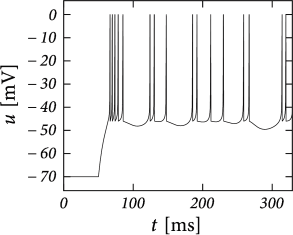
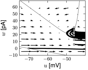
Example: Bursting with a Passive Dendrite and \(I_{M}\)
Suppose that the action potential can be approximated by a one-millisecond pulse at \(0\) mV. Then each spike brings an increase in the dendritic membrane potential. In terms of the current \(w\), the increase is \(b=-aE_0(1-\mathrm{e}^{-1/\tau_w})\). Again, the spike-triggered jump is always negative, leading to spike-triggered facilitation.
The above figures shows an example where we combined a dendritic compartment with the linearized effects of the M-current to result in regular bursting.
The bursting is meditated by the dendritic facilitation which is counterbalanced by the adapting effects of \(I_{M}\).
This example suggests that the dynamics of spike-triggered currents on multiple timescales can be understood in terms of their stereotypical effect on the membrane potential.
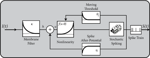
Spike response model (SRM)
We introduced 'filter picture' in section 1.3.5. In this picture, the parameters of the model are replaced by (parametric) functions of time.
In contrast to nonlinear integrate-and-fire models, the SRM has no 'intrinsic' firing threshold but only the sharp numerical threshold for reset.
The subthreshold behavior of the SRM is richer than that of the integrate-and-fire model discussed so far and can account for various aspects of refractoriness and adaptation.
Definition of the SRM
In the framework of SRM the state of a neuron is described by a single variable \(u\) which we interpret as the membrane potential.
After a short current pulse perturbing \(u\), it takes some time before \(u\) returns to rest. The function \(\kappa(s)\) describes the time course of the voltage response to a short current pulse at time \(s=0\). Because the subthreshold behavior of the membrane potential is taken as linear, the voltage response \(h\) to an arbitrary time-dependent stimuating current \(I^{ext}(t')\) is given by the integral \(h(t)=\int_{0}^{\infty} \kappa(s)I^{ext}(t-s) \mathrm{d}s\).
Spike firing is defined by a threshold process. The form of the action potential and the after-potential is described by a function \(\eta\). The evolution of \(u\) is given by \[ u(t)=\sum_{f} \eta(t-t^{(f)})+\int_{0}^{\infty} \kappa(s)I^{ext}(t-s) \mathrm{d}s + u_{rest} \] (6.27)
Introducing the spike train \(S(t)=\sum_{f}^{} \delta(t-t^{(f)})\), (6.27) can be also written as a convolution \[ u(t)=\int_{0}^{\infty} \eta(s)S(t-s) \mathrm{d}s +\int_{0}^{\infty} \kappa(s)I^{ext}(t-s) \mathrm{d}s+u_{rest} \] (6.28)
The threshold \(\theta\) is not fixed, but time-dependent \[ \theta \to \theta(t) \] (6.29)
Firing occurs whenever the membrane potential \(u\) reaches the dynamic threshold \(\theta(t)\) from below \[ t=t^{(f)} \Leftrightarrow u(t)=\theta(t)\ \text{and}\ \frac{\mathrm{d}[u(t)-\theta(t)]}{\mathrm{d}t}>0. \] (6.30)
Example: Dynamic threshold - and how to get rid of it
A standard model of the dynamic threshold is \[ \theta(t)=\theta_0+\sum_{f}^{} \theta_1(t-t^{(f)})=\theta_0+\int_{0}^{\infty} \theta_1(s)S(t-s) \mathrm{d}s \] (6.31)
where \(\theta_0\) is the 'normal' threshold of neuron \(i\) in the absence of spiking. After each output spike, the firing threshold of the neuron is increased by an amount \(\theta_1(t-t^{(f)})\) where \(t^{(f)}<t\) denote the firing times in the past.
For example, during an absolute refractory period \(\Delta^{abs}\), we may set \(\Delta_{\theta}\) for a few milliseconds to a large and positive value so as to avoid any firing and let it relax back to zero over the next few hundred milliseconds.
There is no need to interpret the variable \(u\) as the membrane potential. It is often convenient to transform the variable \(u\) so as to remove the time-dependence of the threshold. \[ \eta(t-t^{(f)}) \to \eta^{eff}(t-t^{(f)})=\eta(t-t^{(f)})-\theta_1(t-t^{(f)}) \] (6.32)
The argument can also be turned the other way round, so as to remove the spike after-potential and only work with a dynamic threshold.


Interpretation of \(\eta\) and \(\kappa\)
(6.27) and (6.30) defines a mathematical model. We'll give a biological interpretation of the terms.
The kernel \(\kappa(s)\) is the linear response of the membrane potential to an input current. It describes the time course of a deviation of the membrane potential from its resting value that is caused by a short current pulse ("impulse response").
The kernel \(\eta\) describes the standard form of an action potential of neuron \(i\) including the negative overshoot which typically follows a spike (the spike afterpotential). Graphically speaking, a contribution \(\eta\) is 'pasted in' each time membrane potential reaches the threshold \(\theta\).
In a simplified model, the form of the action potential may be neglected as long as we keep track of the firing times \(t^{(f)}\). The kernel \(\eta\) describes then simply the 'reset' of the membrane potential to a lower value after the spike at \(t^{(f)}\). \[ \eta(t-t^{(f)})=-\eta_0 \exp \left(-\frac{t-t^{(f)}}{\tau_{recov}}\right) \] (6.33)
with a parameter \(\eta_0>0\) and a recovery time constant \(\tau_{recov}\). The leaky integrate-and-fire model is in fact a special case of the SRM, with parameter \(\eta_0=(\theta-u_{r})\) and \(\tau_{recov}=\tau_m\).
Example: Refractoriness
Absolute refractoriness can be incorporated in the SRM by setting the dynamic threshold during a time \(\Delta^{abs}\) to an extremely high value that cannot be attained.
Relative refractoriness can be mimicked in various ways. - After a spike the firing threshold returns only slowly back to its normal value (increase in firing threshold). - After the spike the membrane potential, and hence \(\eta\), passes through a regime of hyperpolarization (spike after-potential) where the voltage is below the resting potential. During this phase, more stimulation than usual is needed to drive the membrane potential above the threshold. This is equivalent to a transient increase of the firing threshold. - The responsiveness of the neuron is reduced immediately after a spike. In the SRM we can model the reduced responsiveness by making the shape of \(\varepsilon\) and \(\kappa\) depend on the time since the last spike timing \(\hat{t}\).
A slightly more general version of SRM is \[ u(t)=\sum_{f}^{} \eta(t-t^{(f)})+\int_{0}^{\infty} \kappa(t-\hat{t},s)I^{ext}(t-s) \mathrm{d}s+u_{rest}. \] (6.34)
Mapping the Integrate-and-Fire Model to the SRM
Recall that the leaky integrate-and-fire model follows the equation \[ \tau_m \frac{\mathrm{d}u_i}{\mathrm{d}t}=-(u_i-E_0)-R\sum_{k}^{} w_k +RI_i(t) \] (6.35)
\[ \{t_i^{(f)}\} \in \{t | u_i(t)=\theta\}. \] (6.36)
\[
\tau_k \frac{\mathrm{d}w_k}{\mathrm{d}t}=a_k(u_i-E_0)-w_k+\tau_k b_k
\sum_{t^{(f)}}^{} \delta(t-t^{(f)})
\]
(6.37)
Let us consider a short current pulse \(I_i^{out}=-q\delta(t)\) applied to the \(RC\) circuit. Let \(q=C(\theta-u_r)\), the total reset current is \[ I_i^{out}(t)=-C(\theta-u_r)\sum_{f}^{} \delta(t-t_i^{(f)}) \] (6.38)
We add the output current (6.38) on the right-hand side of (6.35), \[ \tau_m\frac{\mathrm{d}u_i}{\mathrm{d}t}=-(u_i-E_0)-R\sum_{k}^{} w_k +RI_i(t)-RC(\theta-u_r) \sum_{f}^{} \delta(t-t_i^{(f)}), \] (6.39)
\[ \tau_k \frac{\mathrm{d}w_k}{\mathrm{d}t}=a_k(u_i-E_0)-w_k+\tau_k b_k \sum_{f}^{} \delta(t-t^{(f)}) \] (6.40)
Now we solve (6.39) and (6.40). - First, we shift the voltage so as to set \(E_0\) to zero. - Second, we calculate the eigenvalues and eigenvectors of the 'free' equations in the absence of input (and therefore no spikes). If there are \(K\) adaptation variables, we have a total of \(K+1\) eigenvalues (including \(\pm \sqrt{R(-a_1-\cdots -a_K)}-1\) and \(-1\) with a multiplicity of \(K-1\)). The associated eigenvectors are \(\mathbf{e}_k\) with components \((e_{k0},\cdots ,e_{kK})^{\mathsf{T}}\). - Third, we express the response to an impulse \(\Delta u=1\) in the voltage (no perturbation in the adaptation variables) in terms of the \(K+1\) eigenvectors: \((1,0,\cdots ,0)^{\mathsf{T}}=\sum_{k=0}^{K} \beta_k \mathbf{e}_k\). - Finally, we express the pulse caused by a reset of voltage and adaptation variables in terms of the eigenvectors \((-\theta+u_r,b_1,\cdots ,b_{K})^{\mathsf{T}}=\sum_{k=0}^{K} \gamma_k \mathbf{e}_k\).
The response to the reset pulses yields the kernel \(\eta\) while the response to voltage pulses yields the filter \(\kappa(s)\) of the SRM \[ u_i(t)=\sum_{f}^{} \eta(t-t_i^{(f)})+\int_{0}^{\infty} \kappa(s)I_i(t-s) \mathrm{d}s, \] (6.41)
with kernels \[ \eta(s)=\sum_{k=0}^{K} \gamma_k e_{k0} \exp (\lambda_k s)\Theta(s), \] (6.42)
\[ \kappa(s)=\sum_{k=0}^{K} \beta_k e_{k0} \exp (\lambda_k s)\Theta(s). \] (6.43)
我大概能理解,但是求导的一些细节不是很了解
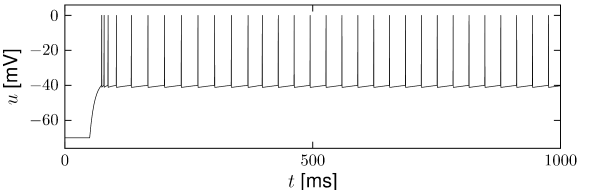
Example: Adaptation and Bursting
Study a leaky integrate-and-fire model with a single slow adaptation variable \(\tau_w\gg \tau_m\) which is coupled to the voltage in the threshold regime (\(a>0\)) and increased during spiking by an amount \(b\).
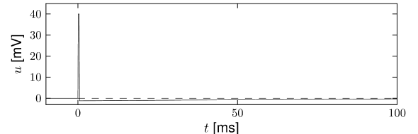
With a parameter \(\delta=\tau_m/\tau_w \ll 1\), the eigenvalues are \(\lambda_1=-\tau_w[1-a\delta]\) and \(\lambda_2=-\tau_w\delta[1+a]\), associated to eigenvectors \(\mathbf{e}_1=(1,a\delta)^{\mathsf{T}}\) and \(\mathbf{e}_2=(1,-1+\delta+a\delta)^{\mathsf{T}}\). The resulting spike after-potential kernel \(\eta(s)\) is shown below. Because of the slow constant \(\tau_w\gg \tau_m\), the kernel \(\eta\) has a long hyperpolarizing tail. The neuron model responds to a step current with adaptation, because of accumulation of hyperpolarizing spike-after potentials over many spikes.
As a second example, consider four adaptation currents with different time constants \(\tau_1<\tau_2<\tau_3<\tau_4\). We assume pure spike-triggered coupling (\(a=0\)) so that the integration of the differential equations of \(w_k\) gives each an exponential current \[ w_k(t)=\sum_{f}^{} b_k \exp \left( -\frac{t-t^{(f)}}{\tau_k}\right) \Theta(t-t^{(f)}) \] (6.44)
Choose as follows: - The time constant of the first current is very short and \(b_1<0\) (inward current) so as to model the upswing of the action potential (a candidate current would be sodium). - A second current (e.g. a fast potassium channel) with a slightly longer time constant is outgoing (\(b_2>0\)) and leads to the downswing and rapid reset of the membrane potential. - The third current, with a time constant of tens of milliseconds is inward (\(b_3<0\)). - The slowest current is again hyperpolarizing (\(b_4>0\)).
The spike after-potential \(\eta\) is shown below.


Because of the depolarizing spike after-potential induced by the inward current \(w_3\), the neuron model responds to a step current of appropriate amplitude with bursts. The bursts end because of the accumulation of the hyperpolarizing effect of the slowest current.
Multi-compartment integrate-and-fire model as a SRM
In this section, we want to show that neurons with a linear dendritic tree and a voltage threshold for spike firing at the soma can be mapped to the SRM.
We study an integrate-and-fire model with a passive dendritic tree described by \(n\) compartments. Membrane resistance, core resistance, and capacity of compartment \(\mu\) are denoted by \(R_{T}^{\mu}\), \(R_{L}^{\mu}\), and \(C^{\mu}\), respectively. The longitudinal core resistance between compartment \(\mu\) and a neighboring compartment \(\nu\) is \(r^{\mu \nu}=(R_{L}^{\mu}+R_{L}^{\nu})/2\). Compartment \(\mu=1\) represents the soma and is equipped with a simple mechanism for spike generation, i.e., with a threshold criterion as in the standard integrate-and-fire model. The remaining dendritic compartments (\(2\leqslant \mu\leqslant n\)) are passive.
Each compartment \(1\leqslant \mu\leqslant n\) of neuron \(i\) may receive input \(I_i^{\mu}(t)\) from presynaptic neurons. As a result of spike generation, there is an additional reset current \(\Omega_i(t)\) at the soma. The membrane potential \(V_i^{\mu}\) of compartment \(\mu\) is given by \[ \frac{\mathrm{d}}{\mathrm{d}t}V_i^{\mu}=\frac{1}{C_i^{\mu}}\left[ -\frac{V_i^{\mu}}{R_{T,i}^{\mu}}-\sum_{\nu}^{} \frac{V_i^{\mu}-V_i^{\nu}}{r_{i}^{\mu \nu}}+I_i^{\mu}(t)-\delta^{\mu 1}\Omega_i(t)\right] \] (6.45)
where the sum runs over all neighbors of compartment \(\mu\). \(\delta^{\mu \nu}\) is the Kronecker symbol. Below we will identify the somatic voltage \(V_i^{1}\) with the potential \(u_i\) of the SRM.
The solution of (6.45) can be formulated by means of Green's functions \(G_{i}^{\mu \nu}(s)\) that describe the impact of an current pulse injected in compartment \(\nu\) on the membrane potential of compartment \(\mu\). The solution is of the form \[ V_{i}^{\mu}(t)=\sum_{\nu}^{} \frac{1}{C_i^{\nu}}\int_{0}^{\infty} G_i^{\mu \nu}(s)[I_i^{\nu}(t-s)-\delta^{\nu 1}\Omega_i(t-s)] \mathrm{d}s. \] (6.46)
这里我完全不理解上面的解法,什么是作用于 compartment \(\nu\) 上的电流对于 compartment \(\mu\) 的影响?另外我对于 Green 函数法解二阶线性齐次常微分方程也有问题:既然 \(f(t)\) 也可以写成 \(\int_{0}^{\infty} \delta(s)f(t-s) \mathrm{d}s\)(积分上下限无所谓),那么为什么在数学物理方法的书上一定要求出非齐次项为 \(\delta(t-s)\) 的关于两个元 \(t,s\) 的 Green 函数 \(G(t,s)\)?
This part is based on Bressloff and Taylor's paper[1].
(6.45) may be written as a linear matrix equation of the form \[ \frac{\mathrm{d}\mathbf{V}}{\mathrm{d}t}=\mathbf{Q} \mathbf{V}(t)+\mathbf{I}(t) \] \[ \mathbf{Q}_{\mu \nu}=-\frac{\delta^{\mu \nu}}{\tau_{\mu}}+\sum_{\nu'}^{} \frac{\delta^{\nu\nu'}}{\tau_{\mu\nu'}} \] \[ \mathbf{I}_{\mu}(t)=\frac{1}{C_i^{\mu}}[I_{i}^{\mu}-\delta^{\mu 1}\Omega_i(t)] \] where \[ \frac{1}{\tau_{\mu}}=\frac{1}{C_i^{\mu}}\left[ \sum_{\nu'}^{} \frac{1}{r_i^{\mu\nu'}}+\frac{1}{R^{\mu}_{T,i}}\right], \quad \frac{1}{\tau_{\mu\nu}}=\frac{1}{C_i^{\mu}r_i^{\mu\nu}} \] (the sum runs over all neighbors of compartment \(\mu\))
The above equation may be solved as (a bit different from (6.46))
\[ V_i^{\mu}(t)=\sum_{\nu}^{} \int_{t_0}^{t} G_i^{\mu\nu}(t-s)I_{\nu}(s) \mathrm{d}s +\sum_{\nu}^{} G_i^{\mu\nu}(t-t_0)V_i^{\nu}(t_0) \quad t\geqslant t_0 \] (maybe the second sum stands for initial condition?) with \[ G_i^{\mu\nu}(t)= [\mathrm{e}^{t \mathbf{Q}}] _{\mu\nu} \]
This coincides with the \(G_i^{\mu\nu}\) in the textbook except for a constant (maybe \(C_i^{\mu}\) or something)
We consider a network made up of a set of neurons described by (6.45) and a simple threshold criterion for generating spikes. We assume that each spike \(t_j^{(f)}\) of a presynaptic neuron \(j\) evokes, for \(t>t_j^{(f)}\), a synaptic current pulse \(\alpha(t-t_j^{(f)})\) into the postsynaptic neuron \(i\). The actual amplitude of the current of the current pulse depends on the strength \(W_{ij}\) of the synapse that connects neuron \(j\) to neuron \(i\). The total input to compartment \(\mu\) of neuron \(i\) is thus \[ I_i^{\mu}(t)=\sum_{j \in \Gamma_i^{\mu}}^{} W_{ij} \sum_{f}^{} \alpha(t-t_j^{(f)}). \] (6.47)
Here, \(\Gamma_i^{\mu}\) denotes the set of all neurons that have a synapse with compartment \(\mu\) of neuron \(i\). The firing times of neuron \(j\) are denoted by \(t_j^{(f)}\).
We assume that spikes are generated at the soma in the manner of the integrate-and-fire model. The reset voltage is \(V_i^{1}=u_r<\theta\). This is equivalent to a current pulse \[ \gamma_i(s)=C_i^{1}(\theta-u_r)\delta(s), \] (6.48)
so that the overall current due to the firing of action potentials at the soma of neuron \(i\) amounts to \[ \Omega_i(t)=\sum_{f}^{} \gamma_i(t-t_i^{(f)}). \] (6.49)
Using the above specializations for the synaptic input current and the somatic reset current the membrane potential (6.46) of compartment \(\mu\) in neuron \(i\) can be written as \[ V_i^{\mu}(t)=\sum_{f}^{} \eta_i^{\mu}(t-t_i^{(f)})+\sum_{\nu}^{} \sum_{j \in \Gamma_i^{\nu}}^{} W_{ij} \sum_{f}^{} \varepsilon_i^{\mu \nu}(t-t_j^{(f)}). \] (6.50)
with \[ \varepsilon_i^{\mu \nu}(s)=\frac{1}{C_i^{\nu}}\int_{0}^{\infty} G_i^{\mu \nu}(s')\alpha(s-s') \mathrm{d}s', \] (6.51) \[ \eta_i^{\mu}(s)=\frac{1}{C_i^{1}}\int_{0}^{\infty} G_i^{\mu 1}(s')\gamma_i(s-s') \mathrm{d}s'. \] (6.52)
The kernel \(\varepsilon_i^{\mu \nu}(s)\) describes the effect of a presynaptic action potential arriving at compartment \(\nu\) on the membrane potential of compartment \(\mu\). Similarly, \(\eta_i^{\mu}(s)\) describes the response of compartment \(\mu\) to an action potential generated at the soma.
The triggering of action potentials depends on the somatic membrane potential only. We define \(u_i=V_i^{1}\), \(\eta_i(s)=\eta_i^{1}(s)\) and, for \(j \in \Gamma_i^{\nu}\), we set \(\varepsilon_{ij}=\varepsilon_i^{1\nu}\). This yields the equation of the SRM \[ u_i(t)=\sum_{f}^{} \eta_i(t-t_i^{(f)})+\sum_{j}^{} W_{ij}\sum_{f}^{} \varepsilon_{ij}(t-t_j^{(f)}). \] (6.53)
Example: Two-compartment integrate-and-fire model
Two compartments are characterized by a somatic capacitance \(C^{1}\) and a dendritic capacitance \(C^{2}=aC^{1}\). The membrane time constant is \(\tau_0=R^{1}C^{1}=R^{2}C^{2}\) and the longitudinal time constant \(\tau_{12}=r^{12}C^{1}C^{2}/(C^{1}+C^{2})\). The neuron fires, if \(V^{1}(t)=\theta\). After each firing the somatic potential is reset to \(u_r\). This is equivalent to a current pulse \[ \gamma(s)=q\delta(s),\tag{6.54} \] where \(q=C^{1}[\theta-u_r]\). The dendrite receives spike trains from other neurons \(j\) and we assume that each spike evokes a current pulse with time course \[ \alpha(s)=\frac{1}{\tau_s}\exp \left(-\frac{s}{\tau_s}\right) \Theta(s). \] (6.55)
With the Green's function we can calculate the response kernels \(\eta_0(s)=\eta_i^{(1)}\) and \(\varepsilon_0(s)=\varepsilon_i^{12}\) as defined in (6.51) and (6.52).
Calculate \(\eta_0(s)\) (omit the subscript \(i\)): \[ \begin{bmatrix} \frac{\mathrm{d}V^{1}}{\mathrm{d}t} \\ \frac{\mathrm{d}V^{2}}{\mathrm{d}t} \end{bmatrix} = \begin{bmatrix} -\frac{1}{C^{1}}\left(\frac{1}{\tau^{12}}+\frac{1}{R^{1}}\right) & \frac{1}{C^{1}\tau^{12}} \\ \frac{1}{aC^{1}\tau^{12}} & -\frac{1}{aC^{1}}\left(\frac{1}{\tau^{12}}+\frac{1}{R^{2}}\right) \end{bmatrix} \begin{bmatrix} V^{1} \\ V^{2} \\ \end{bmatrix} + \begin{bmatrix} -q[\theta-u_r]\delta(t) \\ \frac{1}{\tau_s}\exp \left(-\frac{s}{\tau_s}\right) \Theta(s) \\ \end{bmatrix} \]
which is the form of \(\displaystyle \frac{\mathrm{d}\mathbf{V}}{\mathrm{d}t}=\mathbf{Q} \mathbf{V}(t)+\mathbf{I}(t)\). \[ \mathbf{Q}= \begin{bmatrix} -\frac{a}{(1+a)\tau^{12}}-\frac{1}{\tau_0} & \frac{a}{(1+a)\tau^{12}} \\ \frac{1}{(1+a)\tau^{12}} & -\frac{1}{(1+a)\tau^{12}}-\frac{1}{\tau_0} \\ \end{bmatrix} \]
The eigenvalues of \(\mathbf{Q}\) are \(\displaystyle -\frac{1}{\tau_0}\) and \(\displaystyle -\frac{1}{\tau_0}-\frac{1}{\tau^{12}}\). The corresponding eigenvectors are \((1,1)^{\mathsf{T}}\) and \(\displaystyle (1, -\frac{1}{a})^{\mathsf{T}}\). \[ G^{11}(t)=\left[\int_{0}^{t} \mathrm{e}^{(t-s)\mathbf{Q}} \delta(s) \mathrm{d}s\right]_{11}=[\mathrm{e}^{t \mathbf{Q}}]_{11}=\frac{1}{1+a}\exp \left(-\frac{s}{\tau_0}\right)\left[1+a\exp \left(-\frac{s}{\tau_{12}}\right)\right] \]
So \[ \eta_0(s)=-\frac{1}{C^{1}}\int_{0}^{\infty} G^{11}(s')q\delta(s-s') \mathrm{d}s' \]
Similarly, \[ G^{12}(t)=\frac{a}{1+a}\exp \left(-\frac{t}{\tau_0}\right)\left[1-\exp \left(-\frac{t}{\tau^{12}}\right)\right] \] So \[ \varepsilon_0(s)=\varepsilon^{12}(s)=\frac{1}{C^{2}}\int_{0}^{\infty} G^{12}(s')\frac{1}{\tau_s}\exp \left(-\frac{s-s'}{\tau_s}\right)\Theta(s-s') \mathrm{d}s' \]
We find \[ \eta_0(s)=-\frac{\theta-u_r}{(1+a)}\exp \left(-\frac{s}{\tau_0}\right)\left[1+a\exp \left(-\frac{s}{\tau_{12}}\right)\right], \]
\[ \varepsilon_0(s)=\frac{1}{(1+a)C^{1}}\exp \left(-\frac{s}{\tau_0}\right)\left[\frac{1-\mathrm{e}^{-\delta_1s} }{\tau_s\delta_1}-\exp \left(-\frac{s}{\tau_{12}}\right)\frac{1-\mathrm{e}^{-\delta_2s} }{\tau_s\delta_2}\right], \] (6.56)
with \(\delta_1=\tau_s^{-1}-\tau_0^{-1}\) and \(\delta_2=\tau_s^{-1}-\tau_0^{-1}-\tau_{12}^{-1}\).


The kernel \(\varepsilon_0(s)\) describes the voltage response of the soma to an input at the dendrite. It shows the typical time course of an excitatory or inhibitory postsynaptic potential. The time course of the kernel \(\eta_0(s)\) is a double exponential and reflects the dynamics of the reset in a two-compartment model.
Summary
For the understanding of the Spike Response Model, we introduce
Spike-response model -Scholarpedia http://www.scholarpedia.org/article/Spike-response_model#Leaky_Integrate-and-fire_model
Adaptive exponential integrate-and-fire model -Scholarpedia http://www.scholarpedia.org/article/Adaptive_exponential_integrate-and-fire_model
Exercises
- Timescale of firing rate decay. The characteristic feature of adaptation is that, after the onset of a superthreshold step current, interspike-intervals become successively longer, or, equivalently, that the momentary firing rate drops. The aim is to make a quantitative prediction of the decay of the firing rate of a leak integrate-and-fire model with a single adaptation current.
- Show that the firing rate of (6.7) and (6.8) with constant \(I\), constant \(w\) and \(a=0\) is \[ f(I,w)=-\left[\tau_m \log \left(1-\frac{\theta_{rh}-u_{reset}}{R(I-w)}\right)\right]^{-1}. \] (6.57)
- For each spike (i.e., once per interspike interval), \(w\) jumps by an amount \(b\). Show that for \(I\) constant and \(w\) averaged over one interspike, (6.8) becomes \[ \tau_w \frac{\mathrm{d}w}{\mathrm{d}t}=-w+b\tau_w f(I,w). \] (6.58)
- At time \(t_0\), a strong current of amplitude \(I_0\) is switched on that causes transiently a firing rate \(f\gg \tau_w\). Afterward the firing rate decays. Find the effective time constant of the firing rate for the case of strong input current. Solution: For a) I find that \[ f(I,w)=\left[ \tau \log \left( 1+\frac{\tau_m(\theta_{rh}-u_{reset})}{R(I-w)-\tau_m(\theta_{rh}-u_{rest})} \right) \right]^{-1} \] which must satisfy \[ \theta_{rh}-u_{rest}<\frac{R(I-w)}{\tau_m} \]
- Subthreshold resonance. We study a leaky integrate-and-fire model with a single adaptation variable \(w\).
- Assume \(E_0=u_{rest}\) and cast equation (6.7) and (6.8) in the form of (6.27). Set \(\varepsilon=0\) and calculate \(\eta\) andn \(\kappa\). Show that \(\kappa(t)\) can be written as a linear combination \(\kappa(t)=k_{+}\mathrm{e}^{\lambda_{+}t} +k_{-}\mathrm{e}^{\lambda_{-}t}\) with \[ \lambda_{\pm}=\frac{1}{2\tau_m \tau_w}(-(\tau_m+\tau_w)\pm \sqrt{\tau_m^{2}+\tau_w^{2}-2\tau_m\tau_w(1+2aR)}) \] (6.59) and \[ k_{\pm}=\pm \frac{R(\lambda_{\pm}\tau_w+1)}{\tau_m \tau_w(\lambda_{+}-\lambda_{-})} \] (6.60)
- What are the parameters of (6.7),(6.8) that lead to oscillations in \(\kappa(t)\)?
- What is the frequency of the oscillation?
- Take the Fourier transform of (6.7),(6.8) and find the function \(\hat{R}(w)\) that relates the current \(\hat{I}(w)\) at frequency \(\omega\) to the voltage \(\hat{u}(w)\) at the same frequency, i.e., \(\hat{u}(w)=\hat{R}(w)\hat{I}(w)\). Show that, in the case where \(\kappa\) has oscillations, the function \(\hat{R}(w)\) has a global maximum. What is the frequency where this happens? Solution: (6.7),(6.8) can be expressed as \[ \begin{bmatrix} \frac{\mathrm{d}u}{\mathrm{d}t} \\ \frac{\mathrm{d}w}{\mathrm{d}t} \\ \end{bmatrix} = \begin{bmatrix} -\frac{1}{\tau_m} & -\frac{R}{\tau_m} \\ \frac{a}{\tau_w} & -\frac{1}{\tau_w} \\ \end{bmatrix} \begin{bmatrix} u \\ w \\ \end{bmatrix} + \begin{bmatrix} \frac{E_0+RI(t)}{\tau_m} \\ -\frac{aE_0}{\tau_w} \\ \end{bmatrix} \] Under the assumption that \(I(t)=\delta(t)\), \(E_0=0\), \(w(0)=0\), we get what we want. \(\tau_m^{2}+\tau_w^{2}-2\tau_m\tau_w(1+2aR)<0\) leads to oscillation of \(\kappa(t)\). The frequency is \[ \sqrt{-\tau_m^{2}-\tau_w^{2}+2\tau_m\tau_w(1+2aR)}/2\pi \] For d), \[ \hat{R}(\omega)=\frac{(2\pi i\tau_w \omega+1)R}{-8\pi^{3}\tau_m\tau_w \omega^{2}+1+aR+2\pi i\omega(2\pi \tau_m+\tau_w)} \] > I give up! Ask 1 and 2.
- Integrate-and-fire model with slow adaptation. The aim is to relate the leaky integrate-and-fire model with a singel adaptation variable, defined in (6.7) and (6.8) to the Spike Response Model in the form of (6.27). Adaptation is slow so that \(\tau_m/\tau_w=\delta\ll 1\) and all calculations can be done to first order in \(\delta\).
- Show that the spike after-potential is given by \[ \eta(t)=\gamma_1\mathrm{e}^{\lambda_1t} +\gamma_2 \mathrm{e}^{\lambda_2t} \] (6.61) \[ \gamma_1=\Delta u (1-\delta-\delta a)-b(1+\delta) \] (6.62) \[ \gamma_2=\Delta u -\gamma_1 \] (6.63)
- Derive the input response kernel \(\kappa(s)\). > The initial conditions are \(\eta(0)=\Delta(u)\) and \(w(0)=b\) ? I cannot get the desired result.
- Integrate-and-fire model with time-dependent time constant. Since many channels are open immediately after a spike, the effective membrane time constant after a spike is smaller than the time constant at rest. Consider an integrate-and-fire model with spike-time dependent time constant, i.e., with a membrane time constant \(\tau\) that is a function of the time since the last postsynaptic spike, \[ \frac{\mathrm{d}u}{\mathrm{d}t}=-\frac{u}{\tau(t-\hat{t})}+\frac{1}{C}I^{ext}(t); \] (6.64) As usual, \(\hat{t}\) denotes the last firing time of the neuron. The neuron fires if \(u(t)\) hits a fixed threshold \(\theta\) and integration restarts with a reset value \(u_r\).
- Suppose that the time constant is \(\tau(t-\hat{t})=2\) ms for \(t-\hat{t}<10\) ms and \(\tau(t-\hat{t})=20\) ms for \(t-\hat{t}\geqslant 10\) ms. Set \(u_r=-10\) mV. Sketch the time course of the membrane potential for an input current \(I(t)=q\delta(t-t')\) arriving at \(t'=5\) ms or \(t'=15\) ms. What are the differences between the two cases?
- Integrate (6.64) for arbitrary input with \(u(\hat{t})=u_r\) as initial condition and interpret the result.
- Spike-triggered adaptation currents. Consider a leaky integrate-and-fire model. A spike at time \(t^{(f)}\) generates several adaptation currents \(\mathrm{d}w_k/\mathrm{d}t=-\frac{w_k}{\tau_k}+b_k\delta(t-t^{(f)})\) with \(k=1,\cdots ,K\).
- Calculate the effect of the adaptation current on the voltage.
- Construct a combination of spike-triggered currents that could generates slow adaptation.
- Construct a combination of spike-triggered currents that could generates bursts.
References
- P. C. Bressloff and J. G. Taylor (1994) Dynamics of compartmental model neurons. Neural Networks 7, pp. 1153–1165. ↩︎