Information and Entropy (2)

Communications

Source Model

The source is assumed to produce symbols at a rate of \(R\) symbols per second. The event of the selection of symbol \(i\) will be denoted \(A_i\).

Suppose that each event \(A_i\) is represented by a different codeword \(C_i\) with a length \(L_i\).

An important property of such codewords is that none can be the same as the first portion of another, longer, codeword. A code that obeys this property is called a prefix-condition code, or sometimes an instantaneous code.

Kraft Inequality

An important limitation on the distribution of code lengths \(L_i\) was given by L.G.Kraft, which is known as the Kraft inequality: \[ \sum_{i}^{} \frac{1}{2^{L_i}}\leqslant 1 \tag{6.1} \]

Any valid set of distinct codewords obeys this inequality, and conversely for any proposed \(L_i\) that obey it, a code can be found.

Proof: Let \(L_{max}\) be the length of the longest codeword of a prefix-condition code. There are exactly \(2^{L_{max}}\) different patterns of \(0\) and \(1\) of this length. Thus \[ \sum_{i}^{} \frac{1}{2^{L_{max}}}=1 \tag{6.2} \] where this sum is over these patterns. For each shorter codeword of length \(k(k<L_{max})\) there are exactly \(2^{L_{max}-k}\) patterns that begin with this codeword, and none of those is a valid codeword. In the sum of (6.2) replace the terms corresponding to those patterns by a single term equal to \(1/2^{k}\). The sum is unchanged. Continue this process with other short codewords. Some terms that are not codewords are eliminated. Q.E.D.

Source Entropy

The uncertainty of the identity of the next symbol chosen \(H\) is the average information gained when the next symbol is made known: \[ H=\sum_{i} p(A_i)\log _{2}\left(\frac{1}{p(A_i)}\right) \tag{6.3} \]

This quantity is also known as the entropy of the source. The information rate, in bits per second, is \(H\cdot R\) where \(R\) is the rate at which the source selects the symbols, measured in symbols per second.

Gibbs Inequality

This inequality states that the entropy is smaller than or equal to any other average formed using the same probabilities but a different but a different function in the logarithm. Specifically, \[ \sum_{i}^{} p(A_i)\log _{2}\left(\frac{1}{p(A_i)}\right)\leqslant \sum_{i}^{} p(A_i)\log _{2}\left(\frac{1}{p'(A_i)}\right) \tag{6.4} \] where \(p(A_i)\) is any probability distribution and \(p'(A_i)\) is any other probability distribution, namely, \[ 0\leqslant p'(A_i)\leqslant 1 \tag{6.5} \] and \[ \sum_{i}^{} p'(A_i)\leqslant 1. \tag{6.6} \] As is true for all probability distributions, \[ \sum_{i}^{} p(A_i)=1. \tag{6.7} \] Proof: \[ \begin{aligned} \sum_{i}^{} p(A_i)\log _{2}\left(\frac{1}{p(A_i)}\right)-\sum_{i}^{} p(A_i)\log _{2}\left(\frac{1}{p'(A_i)}\right)&= \sum_{i}^{} p(A_i)\log _{2}\left(\frac{p'(A_i)}{p(A_i)}\right) \\ &\leqslant \log _{2}\mathrm{e} \sum_{i}^{} p(A_i)\left[\frac{p'(A_i)}{p(A_i)}-1\right] \\ &= \log _{2} \mathrm{e} \left(\sum_{i}^{} p'(A_i)-1 \right) \\ &\leqslant 0 \end{aligned} \]

Source Coding Theorem

The codewords have an average length, in bits per symbol, \[ L=\sum_{i}^{} p(A_i)L_i \tag{6.11} \]

The Source Coding Theorem states that the average information per symbol is always less than or equal to the average length of a codeword: \[ H\leqslant L \tag{6.12} \]

This inequality is easy to prove using the Gibbs and Kraft inequalities. Use the Gibbs inequality with \(p'(A_i)=1/2^{L_i}\). Thus \[ \begin{aligned} H&=\sum_{i}^{} p(A_i)\log _{2}\left( \frac{1}{p(A_i)}\right) \\ &\leqslant \sum_{i}^{} p(A_i)\log _{2}\left(\frac{1}{p'(A_i)}\right) \\ &= \sum_{i}^{} p(A_i)\log _{2}2^{L_i}\\ &= \sum_{i}^{} p(A_i)L_i \\ &= L \end{aligned} \]

The Source Coding Theorem can also be expressed in terms of rates of transmission in bits per second by multiplying (6.12) by the symbols per second \(R\): \[ HR\leqslant LR \tag{6.14} \]

Channel Model

If the channel perfectly changes its output state in conformance with its input state, it is said to be noiseless and in that case nothing affects the output except the input.

Suppose that the channel has a certain maximum rate \(W\) at which its output can follow changes at the input.

The binary channel has two mutually exclusive input states.

The maximum rate at which information supplied to the input can affect the output is called the channel capacity \(C=W \log _{2}n\) bits per second. For the binary channel, \(C=W\).

Noiseless Channel Theorem

It may be necessary to provide temporary storage buffers to accommodate bursts of adjacent infrequently occurring symbols with long codewords, and the symbols may not materialize at the output of the system at a uniform rate.

Also, to encode the symbols efficiently it may be necessary to consider several of them together, in which case the first symbol would not be available at the output until several symbols had been presented at the input. Therefore high speed operation may lead to high latency.

Noisy Channel

For every possible input there may be more than one possible output outcome. Denote transition probabilities \(c_{ji}\) the probability of the output event \(B_j\) occuring when event \(A_i\) happens. So \[ 0\leqslant c_{ji}\leqslant 1 \tag{6.15} \] and \[ 1=\sum_{j}^{} c_{ji} \tag{6.16} \] If the channel is noiseless, for each value of \(i\) exactly one of the various \(c_{ji}\) is equal to \(1\) and all others are \(0\). \[ p(B_j|A_i)=c_{ji} \tag{6.17} \] The unconnditional probability of each output \(p(B_j)\) is \[ p(B_j)=\sum_{i}^{} c_{ji}p(A_i) \tag{6.18} \] So by Bayes' Theorem: \[ p(A_i|B_j)=\frac{p(A_i)c_{ji}}{p(B_j)} \tag{6.19} \] The simplest noisy channel is the symmetric binary channel, for which there is a probability \(\varepsilon\) of an error, so \[ \begin{bmatrix} c_{00} & c_{01} \\ c_{10} & c_{11} \\ \end{bmatrix} = \begin{bmatrix} 1-\varepsilon & \varepsilon \\ \varepsilon & 1-\varepsilon \\ \end{bmatrix} \]

Define the information that we have learned about the input as a result of knowing the output as the mutual information.

Before we know the output, our uncertainty \(U_{before}\) about the identity of the input event is he entropy of the input: \[ U_{before}=\sum_{i}^{} p(A_i)\log _{2}\left(\frac{1}{p(A_i)}\right) \tag{6.21} \] After some particular output event \(B_j\) has been observed, the residual uncertainty \(U_{after}(B_j)\) about the input event is: \[ U_{after}(B_j)=\sum_{i}^{} p(A_i|B_j)\log _{2}\left(\frac{1}{p(A_i|B_j)}\right) \tag{6.22} \]

The mutual information \(M\) is defined as the average, over all outputs, of the amount so learned, \[ M=U_{before}-\sum_{j}^{} p(B_j)U_{after}(B_j) \tag{6.23} \] It is not difficult to prove that \(M\geqslant 0\). To prove this, the Gibbs inequality is used, for each \(j\): \[ \begin{aligned} U_{after}(B_j)&=\sum_{i}^{} p(A_i|B_j)\log _{2}\left(\frac{1}{p(A_i|B_j)}\right) \\ &\leqslant \sum_{i}^{} p(A_i|B_j)\log _{2}\left(\frac{1}{p(A_i)}\right) \end{aligned} \] (6.24) So \[ \begin{aligned} \sum_{j}^{} p(B_j)U_{after}(B_j) &\leqslant \sum_{j}^{} p(B_j)\sum_{i}^{} p(A_i|B_j)\log _{2}\left(\frac{1}{p(A_i)}\right) \\ &= \sum_{ji}^{} p(B_j)p(A_i|B_j)\log _{2}\left(\frac{1}{p(A_i)}\right) \\ &= \sum_{ij}^{} p(B_j|A_i)p(A_i)\log _{2}\left(\frac{1}{p(A_i)}\right) \\ &=\sum_{i}^{} p(A_i)\log _{2}\left(\frac{1}{p(A_i)}\right) \\ &=U_{before} \end{aligned} \] (6.25)

Substitution in (6.23) and simplification leads to \[ M=\sum_{j}^{} \left(\sum_{i}^{} p(A_i)c_{ji}\right)\log _{2}\left(\frac{1}{\sum_{i}^{} p(A_i)c_{ji}}\right)-\sum_{ij}^{} p(A_i)c_{ji}\log _{2}\left(\frac{1}{c_{ji}}\right) \] (6.26)

(6.26) was derived for the case where the input "causes" the output. However, such a cause-and-effect relationship is not necessary. The term mutual information suggests that it is just as valid to view the output as causing the input, or to ignore completely the question of what causes what. Two alternate formulas for \(M\) shows that \(M\) can be interpreted in either direction: \[ \begin{aligned} M &= \sum_{i}^{} p(A_i)\log _{2}\left(\frac{1}{p(A_i)}\right)-\sum_{j}^{} p(B_j)\sum_{i}^{} p(A_i|B_j)\log _{2}\left(\frac{1}{p(A_i|B_j)}\right) \\ &= \sum_{j}^{} p(B_j)\log _{2}\left(\frac{1}{p(B_j)}\right)-\sum_{i}^{} p(A_i)\sum_{j}^{} p(B_j|A_i)\log _{2}\left(\frac{1}{p(B_j|A_i)}\right) \end{aligned} \] (6.27)

So (6.26) is easily checked.

Noisy Channel Capacity Theorem

It is more useful to define the channel capacity so that it depends only on the channel, so \(M_{max}\), the maximum mutual information that results from any possible input probability distribution, is used.

Generally speaking, going away from the symmetric case offers few if any advantages in engineered systems, and in particular the fundamental limits given by the theorems in this chapter cannot be evaded through such techniques. Therefore the symmetric case gives the right intuitive understanding.

The channel capacity is defined as \[ C=M_{max}W \tag{6.29} \] where \(W\) is the maximum rate at which the output state can follow changes at the input. Thus \(C\) is expressed in bits per second.

The channel capacity theorem states that: if the input information rate in bits per decond \(D\) is less than \(C\) then it is possible (perhaps by dealing with long sequences of inputs together) to code the data in such a way that the error rate is as low as desired.

The proof is not a constructive proof. However, there is not yet any general theory of how to design codes from scratch.

Reversibility

Some Boolean operations had the property that the input could not be deduced from the output. The \(AND\) and \(OR\) gates are examples. Other operations were reversible——the \(EXOR\) gate, when the output is augmented by one of the two inputs, is an example.

Detail: Communication System Requirements

The systems are characterized by four measures: throughput, latency, tolerance of errors, and tolerance to nonuniform rate (bursts). Throghput is simply the number of bits per second that such a system should, to be successful, accommodate. Latency is the time delay of the message; it could be defined either as the delay of the start of the output after the source begins, or a similar quantity about the end of the message (or, for that matter, about any particular features in the message). The numbers for throughput, in MB (megabytes) or kb (kilobits) are approximate.

---

Channel capacity http://web.archive.org/web/20080126223204/http://www.cs.ucl.ac.uk/staff/S.Bhatti/D51-notes/node31.html

---

Processes

We know the model of a communication system: - Input (Symbols) - Source Encoder - Compressor - Channel Encoder - Channel - Channel Decoder - Expander - Source Decoder - Output(Symbols)

Because each of these steps processes information in some way, it is called a processor and what it does is called a process. The processes we consider here are - Discrete: The inputs are members of a set of mutually exclusive possibilities, only one of which occurs at a time, and the output is one of another discrete set of mutually exclusive events. - Finite: The set of possible inputs is finite in number, as is the set of possible outputs. - Memoryless: The process acts on the input at some time and produces an output based on that input, ignoring any prior inputs. - Nondeterministic: The process may produce a different output when presented with the same input a second time (the model is also valid for deterministic processes). Because the process is nondeterministic the output may contain random noise. - Lossy: It may not be possible to "see" the input from the output, i.e., determine the input by observing the output. Such processes are called lossy because knowledge about the input is lost when the output is created (the model is also valid for lossless processes).

Types of Process Diagrams

We may use block diagram, circuit diagram, probability diagram and information diagram.

Probability Diagrams

We suppose the probability model of a process with \(n\) inputs and \(m\) outputs. The \(n\) inputs are mutually exclusive, as are the \(m\) output states.

For each \(i\) denote the probability that this input leads to the output \(j\) as \(c_{ji}\). Denote the event associated with the selection of input \(i\) as \(A_i\) and the event associated with output \(j\) as \(B_j\).

Example: AND Gates

The \(AND\) gate is deterministic but is lossy.

Example: Binary Channel

Symmetric Binary Channel (SBC), symmetric in the sense that the errors in the two directions are equally likely.

It is possible for processes to introduce noise but have no loss, or vice versa.

Loss of information happens because it is no longer possible to tell with certainty what the input signal is, when the output is observed. Loss shows up in probability diagram where two or more paths converge on the same output.

Noise happens because the output is not determined precisely by the input. Noise shows up in probability diagram where two or more paths diverge from the same input.

Information, Loss, and Noise

We now return to our model of a general discrete memoryless nondeterministic lossy process, and derive formulas for noise, loss, and information transfer.

The information at the input \(I\) is the same as the entropy of this source. \[ I=\sum_{i}^{} p(A_i)\log _{2}\left(\frac{1}{p(A_i)}\right) \] The output information \(J\) can also be expressed in terms of the input probability distribution and the channel transition matrix: \[ \begin{aligned} J &= \sum_{j}^{} p(B_j)\log _{2}\left(\frac{1}{p(B_j)}\right) \\ &= \sum_{j}^{} \left( \sum_{i}^{} c_{ji}p(A_i)\right)\log _{2}\left(\frac{1}{\sum_{i}^{} c_{ji}p(A_i)}\right) \end{aligned} \]

Note that this measure of information at the output \(J\) refers to the identity of the output state, not the input state. If we've got an output state \(B_j\), then the uncertainty of our knowledge of the input state is \[ \sum_{i}^{} p(A_i|B_j)\log _{2}\left(\frac{1}{p(A_i|B_j)}\right) \] So the average uncertainty about the input after learning the output is \[ \begin{aligned} L&=\sum_{j}^{} p(B_j)\sum_{i}^{} p(A_i|B_j)\log _{2}\left(\frac{1}{p(A_i|B_j)}\right) \\ &=\sum_{ij}^{} p(A_i,B_j)\log _{2}\left(\frac{1}{p(A_i|B_j)}\right) \end{aligned} \]

We have denoted this average uncertainty by \(L\) and will call it "loss." In the special case that the process allows the input state to be identified uniquely for each possible output state, the process is "lossless" and \(L=0\).

Denote \(M=I-L\) the "mutual information". This is an important quantity because it is the amount of information tha gets through the process.

Some processes have loss but are deterministic. An example is the \(AND\) logic gate.

There is a quantity similar to \(L\) that characterizes a nondeterministic process, whether or not it has loss. Define the noise \(N\) of a process as the uncertainty in the output, given the input state, averaged over all input states. \[ \begin{aligned} N &= \sum_{i}^{} p(A_i)\sum_{j}^{} p(B_j|A_i)\log _{2}\left(\frac{1}{p(B_j|A_i)}\right) \\ &= \sum_{i}^{} p(A_i)\sum_{j}^{} c_{ji}\log _{2}\left(\frac{1}{c_{ji}}\right) \end{aligned} \]

What may not be obvious, but can be proven easily, is that the mutual information \(M\) plays exactly the same sort of role for noise as it does for loss. Since \[ J=\sum_{i}^{} p(B_j)\log _{2}\left(\frac{1}{p(B_j)}\right) \] we have \[ M=J-N \tag{7.24} \] It follows from these results that \[ J-I=N-L \tag{7.27} \]

Example: Symmetric Binary Channel

For the SBC with bit error probability \(\varepsilon\), these formulas can be evaluated, even if the two input probabilities \(p(A_0)\) and \(p(A_1)\) are not equal. If they happen to be equal (each 0.5), then \[ I=1\ \text{bit} \] \[ J=1\ \text{bit} \] \[ L=N=\varepsilon \log _{2}\left(\frac{1}{\varepsilon}\right)+(1-\varepsilon) \log _{2}\left(\frac{1}{1-\varepsilon}\right) \] \[ M=1-\varepsilon \log _{2}\left(\frac{1}{\varepsilon}\right)-(1-\varepsilon)\log _{2}\left(\frac{1}{1-\varepsilon}\right) \]

Deterministic Examples

p88-89

Error Correcting Example

p89-90

Capacity

Call \(W\) the maximum rate at which the input state of the process can be detected at the output. Then the rate at which information flows through the process can be as large as \(WM\). However, this product is not a property of the process itself, but on how it is used. The process capacity \(C\) is defined as \[ C=WM_{max} \tag{7.32} \]

Information Diagrams

p91

Cascaded Processes

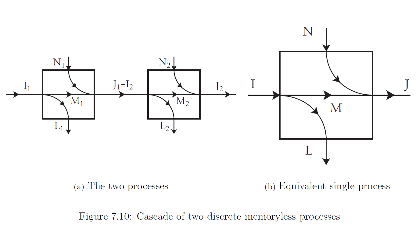
Consider two processes in cascade. This term refers to having the output from one process serve as the input to another process.

The matrix of transition probabilities is merely the matrix product of the two transition probability matrices for process 1 and process 2.

Now we seek formulas for \(I,J,L,N\) and \(M\) of the overall process in terms of the corresponding quantities for the component processes.

\(I=I_1\) and \(J=J_2\). \(L\) and \(N\) cannot generally be found exactly from \(L_1,L_2,N_1\) and \(N_2\), it is possible to find upper and lower bounds for them. \[ L-N=(L_1+L_2)-(N_1+N_2)\tag{7.33} \] The loss \(L\) for the overall process is not always equal to the sum of the losses for the two components \(L_1+L_2\), but instead \[ 0\leqslant L_1\leqslant L\leqslant L_1+L_2 \tag{7.34} \] so that the loss is bound from above and below. Also, \[ L_1+L_2-N_1\leqslant L\leqslant L_1+L_2 \tag{7.35} \] so that if the first process is noise-free then \(L\) is exactly \(L_1+L_2\).

There are similar formulas for \(N\) in terms of \(N_1+N_2\): \[ 0\leqslant N_2\leqslant N\leqslant N_1+N_2 \tag{7.36} \] \[ N_1+N_2-L_2\leqslant N\leqslant N_1+N_2 \tag{7.37} \] Similar formulas for the mutual information of the cascade \(M\) follow from these results: \[ M_1-L_2\leqslant M\leqslant M_1\leqslant I \tag{7.38} \] \[ M_1-L_2\leqslant M\leqslant M_1+N_1-L_2 \tag{7.39} \] \[ M_2-N_1\leqslant M\leqslant M_2\leqslant J \tag{7.40} \] \[ M_2-N_1\leqslant M\leqslant M_2+L_2-N_1 \tag{7.41} \] Other formulas for \(M\) are easily derived from \(0\leqslant M\leqslant I\) applied to the first process and the cascade, and \(M=J-N\) applied to the second process and the cascade: \[ \begin{aligned} M &= M_1+L_1-L \\ &=M_1+N_1+N_2-N-L_2 \\ &=M_2+N_2-N \\ &=M_2+L_2+L_1-L-N_1 \end{aligned} \] where the second formula in each case comes from the use of (7.33).

\(M\) cannont exceed either \(M_1\) or \(M_2\). If the second process is lossless, \(L_2=0\) and then \(M=M_1\). Similarly if the first process is noiseless, then \(N_1=0\) and \(M=M_2\).

The channel capacity \(C\) of the cascade satisfies \(C\leqslant C_1\) and \(C\leqslant C_2\). However, other results relating the channel capacities are not a trivial consequence of the formulas above.

Inference

Estimation

We now try to determine the input event when the output has been observed. This is the case for communication systems and memory systems.

The conditional output probabilities \(c_{ji}\) are a property of the process, and do not depend on the input probabilities \(p(A_i)\).

The unconditional probability \(p(B_j)\) of each output event \(B_j\) is \[ p(B_j)=\sum_{i}^{} c_{ji}p(A_i) \tag{8.1} \] and \[ p(A_i,B_j)=p(A_i)c_{ji} \tag{8.2} \] so \[ p(A_i|B_j)=\frac{p(A_i)c_{ji}}{p(B_j)} \tag{8.3} \] If the process has no loss (\(L=0\)) then for each \(j\) exactly one of the input events \(A_i\) has nonzero probability, and therefore its probability \(p(A_i|B_j)\) is \(1\).

We know \[ U_{before}=\sum_{i}^{} p(A_i)\log _{2}\left(\frac{1}{p(A_i)}\right) \] and the residual uncertainty after some particular output event is \[ U_{after}(B_j)=\sum_{i}^{} p(A_i|B_j)\log _{2}\left(\frac{1}{p(A_i|B_j)}\right) \]

The question is whether \(U_{after}(B_j)\leqslant U_{before}\). The answer is often, but not always, yes.

On average, out uncertainty about the input state is never increased by learning something about the output state.

Non-symmetric Binary Channel

For a rare family genetic disease,

	\(p(A)\)	\(p(B)\)	\(I\)	\(L\)	\(M\)	\(N\)	\(J\)
Family history	0.5	0.5	1.00000	0.11119	0.88881	0.11112	0.99993
Unknown Family history	0.9995	0.0005	0.00620	0.00346	0.00274	0.14141	0.14416

Inference Strategy

One simple strategy for inference is "maximum likelihood". However, sometimes it does not work at all (rare family genetic disease test).

Principle of Maximum Entropy: Simple Form

Before the Principle of Maximum Entropy can be used the problem domain needs to be set up. It is not assumed in this step which particular state the system is in (or which state is actually "occupied"); indeed it is assumed that we do not know and cannot know this with certainty, and so we deal instead with the probability of each of the states being occupied.

Berger's Burgers

The Principle of Maximum Entropy will be introduced by means of an example. A fast-food restaurant, Berger's Burgers, offers three meals: burger, chicken, and fish. The price, Calorie count, and probability of each meal being delivered cold are as listed below.

Item	Entree	Cost	Calories	Probability of arriving hot	probability of arriving cold
Value Meal 1	Burger	1.00	1000	0.5	0.5
Value Meal 2	Chicken	2.00	600	0.8	0.2
Value Meal 3	Fish	3.00	400	0.9	0.1

Probabilities

If we do not know the outcome we may still have some knowledge, and we use probabilities to express this knowledge.

Entropy

Our uncertainty is expressed as \[ S=p(B)\log _{2}\left(\frac{1}{p(B)}\right)+p(C)\log _{2}\left(\frac{1}{p(C)}\right)+p(F)\log _{2}\left(\frac{1}{p(F)}\right) \] In the context of physical systems this uncertainty is known as the entropy. In communication systems the uncertainty regarding which actual message is to be transmitted is also known as the entropy of the source.

In general the entropy, because it is expressed in terms of probabilities, depends on the observer. One person may have different knowledge of the system from another, and therefore would calculate a different numerical value for entropy.

The Principle of Maximum Entropy is used to discover the probability distribution which leads to the highest value for this uncertainty, thereby assuring that no information is inadvertently assumed. The resulting probability distribution is not observer-dependent.

Constraints

If we have additional information then we ought to be able to find a probability distribution that is better in the sense that it has less uncertainty.

We consider we know the expected value of some quantity (the Principle of Maximum Entropy can handle multiple constraints but the mathematical procedures and formulas become more complicated) If there is an attribute for which each of the states has a value \(g(A_i)\) and for which we know the actual value \(G\), then we should consider only those probability distributions for which the expected value is equal to \(G\).

\[ G=\sum_{i}^{} p(A_i)g(A_i) \tag{8.15} \]

In the case that the average cost is 1.75, \(S\) attains its maximum when \(p(B)=0.466\), \(p(C)=0.318\), \(p(C)=0.318\), and \(S=1.517\) bits.