Neuronal Dynamics (4)

Dimensionality Reduction and Phase Plane Analysis

The online version of this chapter:

---

Chapter 4 Dimensionality Reduction and Phase Plane Analysis https://neuronaldynamics.epfl.ch/online/Ch4.html

---

Threshold effects

In this section we use current pulses ans steps in order to explore the threshold behavior of the Hodgkin-Huxley model.

Pulse Input

The threshold depends on the stimulation protocol.

Step Current Input

We study the response of the Hodgkin-Huxley model to a step current of the form \[ I(t)=I_1+\Delta I \mathscr{H}(t) \] where \(\mathscr{H}\) denotes the Heaviside step function.

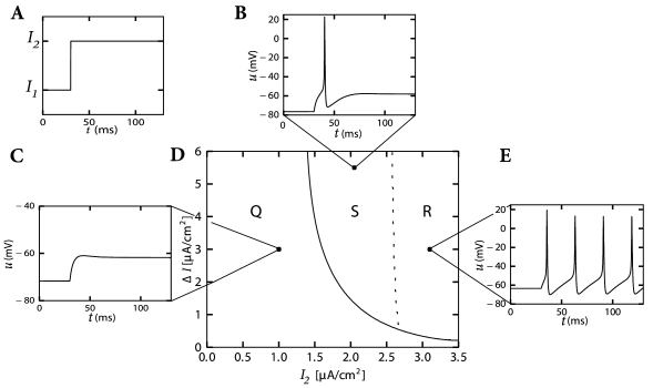
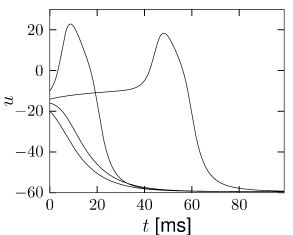
When probing with step currents, there is neither a unique current threshold for spike initiation nor for repetitive firing. The trigger mechanism for action potentials depends not only on \(I_2\) but also on the size of the current step \(\Delta I\).

Biologically, the dependence upon the step size arises from the different time constants of activation and inactivation of the ion channels. We'll see it below.

Reduction to two dimensions

General approach

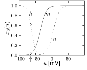
Note that the time scale of \(m\) is much faster than \(n\) and \(h\). Moreover, \(m\) is fast compared to the membrane time constant \(\tau=C/g_{L}\) of a passive membrane, which characterizes the evolution of the voltage \(u\) when all channels are closed. So we may treat \(m\) as an instantaneous variable, therefore it can be replaced by its steady-state value, \(m(t) \to m_0[u(t)]\). (quasi steady state approximation)

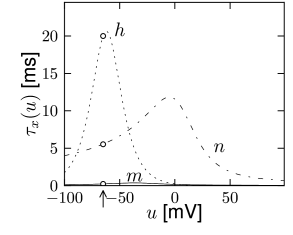
Note that the time constants \(\tau_n(u)\) and \(\tau_{h}(u)\) have similar dynamics over the voltage \(u\). Moreover, the graphs of \(n_0(u)\) and \(1-h_0(u)\) are also similar.

We use a linear approximation \((b-h)\thickapprox an\) with some constants \(a,b\) and set \(w=b-h=an\). With \(h=b-w\), \(n=w/a\), and \(m=m_0(u)\), equations (2.4)-(2.5) become \[ C\frac{\mathrm{d}u}{\mathrm{d}t}=-g_{Na}[m_0(u)]^{3}(b-w)(u-E_{Na})-g_{K}(\frac{w}{a})^{4}(u-E_{K})-g_{L}(u-E_{L})+I, \tag{4.3} \] or \[ \frac{\mathrm{d}u}{\mathrm{d}t}=\frac{1}{\tau}[F(u,w)+RI], \tag{4.4} \] with \(R=g_{L}^{-1}\), \(\tau=RC\) and some function \(F\). We also have \[ \frac{\mathrm{d}w}{\mathrm{d}t}=\frac{1}{\tau_{w}}G(u,w), \tag{4.5} \]

Example: Morris-Lecar model

The Morris-Lecar equations read \[ C\frac{\mathrm{d}u}{\mathrm{d}t}=-g_1 \hat{m}_0(u)(u-V_1)-g_2 \hat{w}(u-V_2)-g_{L}(u-V_{L})+I, \tag{4.6} \] \[ \frac{\mathrm{d}\hat{w}}{\mathrm{d}t}=-\frac{1}{\tau(u)}[\hat{w}-w_0(u)]. \tag{4.7} \]

(4.6) doesn't have the factor \((b-w)\) which closes the channel for high voltage. Another difference is that neither \(\hat{m}_0\) nor \(\hat{w}\) have exponents. In the following we consider (4.6) and (4.7) as a model in its own right and drop the hats over \(m_0\) and \(w\).

It's reasonable to approximate the voltage dependence by \[ m_0(u)=\frac{1}{2}\left[ 1+ \tanh \left( \frac{u-u_1}{u_2}\right)\right] \tag{4.8} \] \[ w_0(u)=\frac{1}{2}\left[ 1+ \tanh \left( \frac{u-u_3}{u_4}\right)\right] \tag{4.9} \] with parameters \(u_1,\cdots ,u_4\), and to approximate the time constant by \[ \tau(u)=\frac{\tau_{w}}{\cosh(\frac{u-u_3}{2u_4})} \tag{4.10} \] with a further parameter \(\tau_{w}\).

Example: FitzHugh-Nagumo model

FitzHugh and Nagumo obtained sharp pulse-like oscillations reminiscent of trains of action potentials by defining the function \(F(u,w)\) and \(G(u,w)\) as
\[ \begin{cases} F(u,w)=u-\frac{1}{3}u^{3}-w, \\ G(u,w)=b_0+b_1u-w, \end{cases} \tag{4.11} \]

where \(u\) is the membrane voltage and \(w\) is a recovery variable.

Mathematical steps

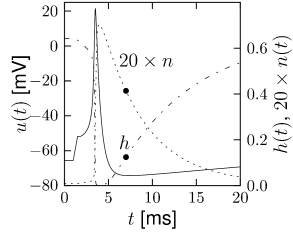
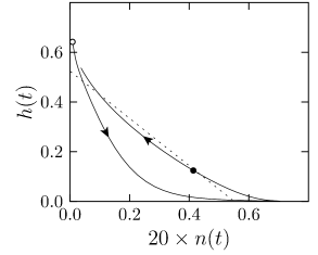
The overall aim of the approach is to replace the variables \(n\) and \(h\) in the Hodgkin-Huxley model by a single effective variable \(w\). During an action potential, the variables \(n(t)\) and \(h(t)\) stay close to a straight line.

A minimal condition for the projection is that the approximation is perfect while the neuron is at rest. First, we introduces new variables \[ x=n-n_0(u_{rest}) \tag{4.12} \] \[ y=h-h_0(u_{rest}). \tag{4.13} \] At rest, we have \(x=y=0\).

Second, the points \((n_0(u),h_0(u))\) as a function of \(u\) define a curve. The slope of the curve at \(u=u_{rest}\) yields the rotation angle \(\alpha\) via \[ \tan \alpha=\frac{ \frac{\mathrm{d}h_0}{\mathrm{d}u}\big |_{u_{rest}}}{ \frac{\mathrm{d}n_0}{\mathrm{d}u}\big |_{u_{rest}}} \] Rotate the coordinates \[ \begin{pmatrix} z_1 \\ z_2 \\ \end{pmatrix} = \begin{pmatrix} \cos \alpha & \sin \alpha \\ -\sin \alpha & \cos \alpha \\ \end{pmatrix} \begin{pmatrix} x \\ y \\ \end{pmatrix}. \]

The inverse transform \[ \begin{pmatrix} x \\ y \\ \end{pmatrix} = \begin{pmatrix} \cos \alpha & -\sin \alpha \\ \sin \alpha & \cos \alpha \\ \end{pmatrix} \begin{pmatrix} z_1 \\ z_2 \\ \end{pmatrix}. \]

Project \((n,h)\) to the line expanded by \(z_1\), namely, \(z_2=0\). \[ n'=n_0(u_{rest})+z_1\cos \alpha, \tag{4.17} \] \[ h'=h_0(u_{rest})+z_1\sin \alpha. \tag{4.18} \]

From (4.15) we find \[ \frac{\mathrm{d}z_1}{\mathrm{d}t}=\cos \alpha \frac{\mathrm{d}n}{\mathrm{d}t}+\sin \alpha \frac{\mathrm{d}h}{\mathrm{d}t}. \tag{4.19} \] Since \[ \frac{\mathrm{d}n}{\mathrm{d}t}=-\frac{1}{\tau_n(u)}[n-n_0(u)] \] and an similar equation for \(h\), we have \[ \frac{\mathrm{d}z_1}{\mathrm{d}t}=-\cos \alpha \frac{z_1 \cos \alpha+n_0(u_{rest})-n_0(u)}{\tau_{n}(u)}- \sin \alpha \frac{z_1 \sin \alpha+h_0(u_{rest})-h_0(u)}{\tau_{h}(u)}. \tag{4.20} \] which is of the form \(\mathrm{d}z_1/\mathrm{d}t=G(u,z_1)\), as desired.

It is convenient to rescale \(z_1\) and define \[ w=- n_0(u_{rest})\tan \alpha-z_1 \sin \alpha. \tag{4.21} \] If we introduce \(a=-\tan \alpha\) and \(b=a n_0(u_{rest})+h_0(u_{rest})\), we find from (4.17) \(n'=w/a\) and from (4.18) \(h'=b-w\). We also have \(\mathrm{d}w/\mathrm{d}t=G(u,w)\). Actually, \[ \frac{\mathrm{d}w}{\mathrm{d}t}=-\frac{1}{\tau(u)}[w-w_0(u)]. \tag{4.22} \] with \[ w_0(u)=-\sin \alpha[n_0(u)\cos \alpha+h_0(u)\sin \alpha-b\sin \alpha] \tag{4.23} \] In practice, \(w_0(u)\) and \(\tau(u)\) can be fitted by (4.9) and (4.10), respectively.

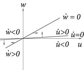
Phase plane analysis

We know \[ \begin{pmatrix} \Delta u \\ \Delta w \\ \end{pmatrix} = \begin{pmatrix} \dot{u} \\ \dot{v} \\ \end{pmatrix} \Delta t. \tag{4.24} \]

Case A is stable, Case C and D are unstable. Stability in case B cannot be decided with the information available from the picture alone. C and D are saddle points.

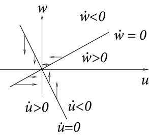
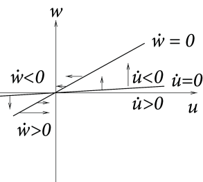
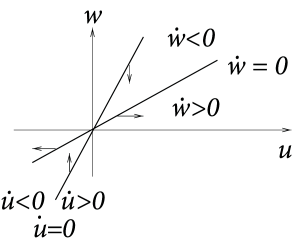
Nullclines

The set of points with \(\dot{u}=0\) is called the \(u-\)nullcline.

Stability of Fixed Points

The local stability of a fixed point \((u_{FP},w_{FP})\) is determined by linearization of the dynamics at the intersection. With \(\mathbf{x}=(u-u_{FP},w-w_{FP})^{\mathsf{T}}\), we have after the linearization \[ \frac{\mathrm{d}}{\mathrm{d}t}\mathbf{x}= \begin{pmatrix} F_u & F_w \\ G_u & G_w \\ \end{pmatrix} \mathbf{x}\tag{4.25} \]

Stability of the fixed point \(\mathbf{x}=0\) in (4.25) requires that the real part of both eigenvalues be negative. The necessary and sufficient condition for stability is therefore \[ F_u+G_w<0 \quad \text{and} \quad F_u G_w-F_w G_u>0. \] If \(F_u G_w-F_w G_u<0\), the fixed point is then called a saddle point.

Example: Linear model

\[ \dot{u}=au-w \\ \dot{w}=\varepsilon(bu-w), \tag{4.27} \] with positive constants \(b,\varepsilon>0\). The \(u-\)nullcline is \(w=au\), the \(w-\)nullcline is \(w=bu\). For the moment we assume \(a<0\).

For the sake of completeness we also study the linear system \[ \dot{u}=-au+w \\ \dot{w}=\varepsilon(bu-w), 0<a<b, \tag{4.28} \] with positive constants \(a,b\), and \(\varepsilon\).

Recall the theorem of Poincare-Bendixson.

In dimensionless variables the FitzHugh-Nagumo model is \[ \frac{\mathrm{d}u}{\mathrm{d}t}=u-\frac{1}{3}u^{3}-w+I \tag{4.29} \] \[ \frac{\mathrm{d}w}{\mathrm{d}t}=\varepsilon(b_0+b_1u-w). \tag{4.30} \] Time is measured in units of \(\tau\) and \(\varepsilon=\tau/\tau_w\) is the ratio of the two time scales.

Type I and Type II neuron models

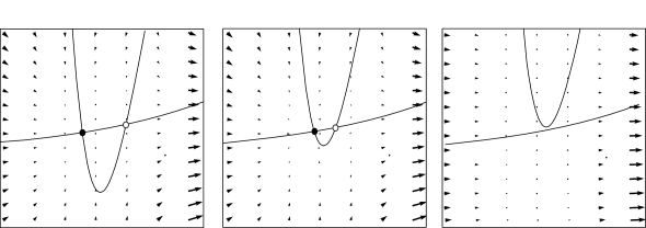
The onset of repetitive firing under constant current injection is characterized by a minimal current \(I_{\theta}\), also called the rheobase current. Mathematically speaking, the point \(I_{\theta}\) where the transition in the number or stability of fixed points occurs is called a bifurcation point and \(I\) is the bifurcation parameter.

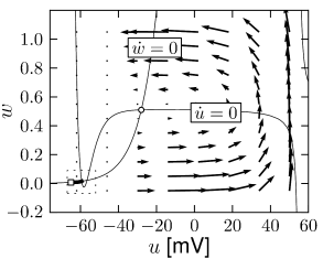
Type I Models and Saddle-Node-onto-Limit-Cycle Bifurcation

Neuron models with a continuous gain function. Mathematically, a saddle-node-onto-limit-cycle bifurcation generically gives rise to a type I behavior.

Example: Morris-Lecar model

Depending on the choice of parameters, the Morris-Lecar model is of either type I or type II.

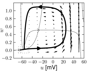
Example: Hodgkin-Huxley Model Reduced to Two Dimensions

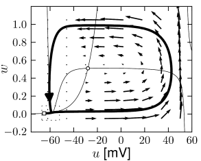
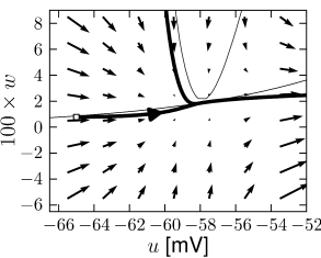
(4.14)

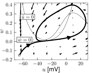
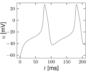
Type II Models and Saddle-Node-off-Limit-Cycle Bifurcation

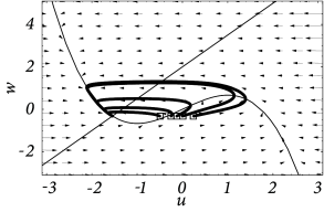
There is no reason why a limit cycle should appear directly at the bifurcation point - it can also exist before the bifurcation point is reached. In this case, the limit cycle does not pass through the ruins of the fixed point and therefore has finite frequency. This gives rise to a type II neuron model. (Saddle-Node-off-Limit-Cycle)

Example: Hodgkin-Huxley Model Reduced to Two Dimensions

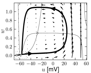
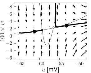
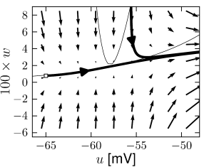
(4.15)

(4.15) shows the same neuron model as (4.14) except for one single change in parameter: the time scale \(\tau_{w}\) in (4.5) for the \(w-\)dynamics is slightly faster.

Example: Saddle-node without limit cycle

Not all saddle-node bifurcations lead to a limit cycle. If the slope of the \(w-\)nullcline of the FitzHugh-Nagumo model defined in (4.29) and (4.30) is smaller than one, it is possible to have three fixed points, one of them unstable and the other two stable. The system is therefore bistable. If \(I>0\) is big enough so that the left stable fixed point and the saddle merge and disappear. Since the right fixed point remains stable, no oscillation occurs.

Type II Models and Hopf Bifurcation

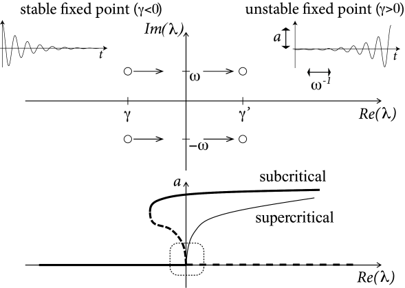
From the solution of the stability problem in (4.25) we know that the eigenvalues \(\lambda_{+/-}\) form a complax conjugate pair with a real part \(\gamma\) and a imaginary part \(+/-\omega\) (Fig. 4.16). The fixed point is stable if \(\gamma<0\). At the transition point, the real part vanishes and the eigenvalues are \[ \lambda_{\pm}=\pm i \sqrt{F_u G_w-G_u F_w}. \tag{4.31} \] These eigenvalues correspond to an oscillatory solution with a frequency given by \(\omega=\sqrt{F_u G_w-G_u F_w}\).

(4.16)

Whenever we have a Hopf bifurcation, be it subcritical or supercritical, the limit cycle starts with finite frequency.

In a supercritical Hopf bifurcation, the amplitude of the oscillation grows with the stimulation \(I\). Such periodic oscillations of small amplitude should be intepreted as spontaneous subthreshold oscillations.

Only models with a subcritical Hopf-bifurcation give rise to large-amplitude oscillations close to the bifurcation point.

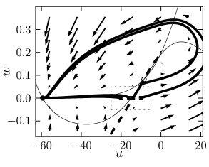
Example: FitzHugh-Nagumo model

In Fig. 4.10, if the slope of the \(w-\)nullcline is larger than one, there is only one fixed point, whatever \(I\). With increasing current \(I\), the fixed point moves to the right. Eventually it loses stability via a Hopf bifurcation.

Threshold and excitability

The Hodgkin-Huxley model does not have a clear-cut firing threshold.

For stimulation with a short current pulse of variable amplitude, models with saddle-node bifurcation (on or off a limit cycle) indeed have a threshold whereas models where firing arises via a Hopf bifurcation have not. However, even models with Hopf bifurcation can show threshold-like behavior for current pulse if the dynamics of \(w\) are consideraby slower than that of \(u\).

Type I models

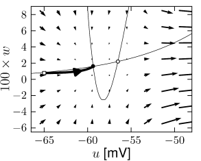
The stable manifold of an saddle point. All trajectories with initial condition to the right of the stable manifold must make a detour around the unstable fixed point before they can reach the stable fixed point. Trajectories with initial conditions to the left of the stable manifold return immediately toward the stable fixed point.

The stable manifold acts as a threshold for spike initiation, if the neuron model is probed with a isolated current pulse.

Example: Canonical type I model

Consider the one-dimensional model \[ \frac{\mathrm{d}\phi}{\mathrm{d}t}=q(1-\cos \phi)+I(1+\cos \phi) \tag{4.32} \] where \(q>0\) is a parameter and \(I\) with \(0<\lvert I \rvert <q\) the applied current. The variable \(\phi\) is the phase along the limit cycle trajectory. Formally, a spike is said to occur whenever \(\phi=\pi\).

For \(I<0\), the phase equation \(\mathrm{d}\phi/\mathrm{d}t\) has two fixed points. The resting state is at the stable fixed point \(\phi=\phi_r\). The unstable fixed point at \(\phi=\theta\) acts as a threshold.

For all currents \(I>0\), we have \(\mathrm{d}\phi/\mathrm{d}t>0\), so that the system is circling along the limit cycle. For \(I \to 0\), the velocity along the trajectory around \(\phi=0\) tends to zero. Therefore the frequency of the oscillation \(\nu=1/T(I)\) decreases to zero.

Hopf Bifurcations

There is a continuum of trajectories.

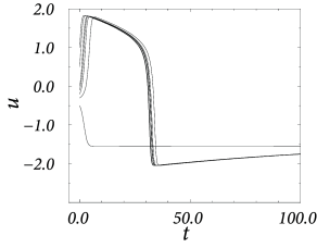
Nevertheless, if the time scale of the \(u\) dynamics is much faster than that of the \(w-\)dynamics, then there is a critical regime where the sensitivity to the amplitude of the input current pulse can be extremely high.

In models with Hopf bifurcation, the peak of the response is always reached with roughly the same delay, independently of the size of the input pulse. It is the amplitude of the response that increases rapidly but continuously.

Separation of time scales and reduction to one dimension

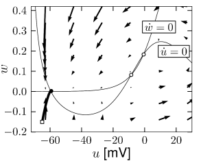
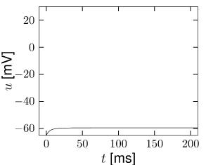
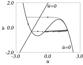
We measure time in units of \(\tau\) and take \(R=1\) in (4.4) and (4.5). Then \[ \frac{\mathrm{d}u}{\mathrm{d}t}=F(u,w)+I \tag{4.33} \] \[ \frac{\mathrm{d}w}{\mathrm{d}t}=\varepsilon G(u,w) \tag{4.34} \] where \(\varepsilon=\tau/\tau_w\). If \(\tau_w\gg \tau\), then \(\varepsilon\ll 1\). In this situation the time scale the governs the evolution of \(u\) is much faster than that of \(w\). In the mathematical literature the limit of \(\varepsilon \to 0\) is called 'singular perturbation'. Oscillatory behavior for small \(\varepsilon\) is called a 'relaxation oscillation'. Trajectories slowly follow the \(u-\)nullcline, except at the knees of the nullcline where they jump to a different branch.

In the above figure the middle branch of the \(u-\)nullcline (where \(\dot{u}>0\)) acts as a threshold for spike initiation.

We can exploit the separation of times scales for a further reduction of the two-dimensional system of equations to a single variable. An input current \(I(t)\) acts on the voltage dynamics, but has no direct influence on the variable \(w\). Moreover, in the limit of \(\varepsilon\ll 1\), the influence of the voltage \(u\) on the \(w-\)variable via (4.34) is negligible. Hence, we can set \(w=w_{rest}\) and summarize the voltage dynamics of spike initiation by a single equation \[ \frac{\mathrm{d}u}{\mathrm{d}t}=F(u,w_{rest})+I. \tag{4.35} \]

Example: Piecewise linear nullclines

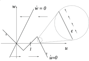
\[ \frac{\mathrm{d}u}{\mathrm{d}t}=f(u)-w+I \tag{4.36} \] \[ \frac{\mathrm{d}w}{\mathrm{d}t}=\varepsilon(bu-w) \tag{4.37} \]

with \(f(u)=au\) for \(u<0.5\), \(f(u)=a(1-u)\) for \(0.5< u< 1.5\) and \(f(u)=c_0+c_1u\) for \(u>1.5\) where \(a\),\(c_1<0\) are parameters and \(c_0=-0.5a-1.5c_1\). Furthermore, \(b>0\) and \(0<\varepsilon\ll 1\).

The rest state is at \(u=w=0\). \(u=1\) acts as a threshold. Let us now suppose that neuron receives a weak and constant background current during our threshold-search experiments. A constant current shifts the \(u-\)nullcline vertically upward. Hence the point where \(\dot{u}=0\) shifts leftward and therefore the voltage threshold for pulse stimulation sits now at a lower value.